
Real-time nowcasting: right-truncation vs the reporting triangle
In real time the most recent days of a surveillance series are incomplete. A case with reference day
This package corrects right-truncation two ways, and this tutorial fits and compares both on the same simulated data. RightTruncate is the marginal correction. It keeps only each reference day's observed-so-far total and scales the expected count by the reporting-delay CDF, the EpiNow2-style CDF-scaling nowcast. ReportTriangle is the joint correction. It keeps the full reference-day × reporting-delay triangle and scores it cell by cell, the epinowcast-style nowcast. The two share one reporting-delay kernel, so the triangle's observed row-sums are exactly the observed-so-far totals the marginal correction conditions on. Both leave the renewal infection process and its latent
The two corrections
The infection pipeline produces
Summing the joint model's observed cells over
The renewal model
Both corrections wrap the same composed renewal model as the renewal tutorial, an autoregressive Renewal infection process observed with a NegativeBinomialError.
using ComposableTuringIDModels, Distributions, Random, Turing, Mooncake
using ADTypes: AutoMooncake
using CSV, DataFrames
Random.seed!(20240625)

adt = AutoMooncake(; config = nothing)

latent = AR(
    damp = [truncated(Normal(0.8, 0.05), 0, 1)],
    init = [Normal(0.0, 0.25)],
    ϵ_t = HierarchicalNormal(std = HalfNormal(0.1)))
renewal = Renewal(; generation_time = Gamma(1.4, 1 / 0.38),
    rt = latent, initialisation = Normal(log(1.0), 1.0))
error = NegativeBinomialError(cluster_factor = HalfNormal(0.1))
Simulate a reporting triangle
We take the fully-reported Italy confirmed-case series as the eventual totals, split each day's total across reporting delays with the delay PMF, then mask the cells not yet reported at ReportingPMF discretises the reporting delay with the same CensoredDistributions.jl path the rest of the package uses.
datapath = joinpath(pkgdir(ComposableTuringIDModels),
    "docs", "src", "tutorials", "data", "italy_data.csv")
italy = CSV.read(datapath, DataFrame)
n = 45
eventual = italy.confirm[1:n]                 # eventual (complete) totals

reporting_delay = LogNormal(1.6, 0.5)         # mean ≈ 5.6 days
delay_pmf = ReportingPMF(reporting_delay; D = 10)
pmf = delay_pmf.pmf                            # delays 0 … Dmax
Dmax = length(pmf) - 1
Split each reference day's eventual total across delays with a multinomial draw, then keep only the cells reported by
full_triangle = reduce(vcat,
    (permutedims(rand(Multinomial(eventual[t], pmf))) for t in 1:n))
mask = [t + d <= n for t in 1:n, d in 0:Dmax]
reported_triangle = full_triangle .* mask
observed_so_far = vec(sum(reported_triangle, dims = 2))
(complete_tail = eventual[(end - 4):end],
    truncated_tail = observed_so_far[(end - 4):end])
(complete_tail = [4782, 4668, 4585, 4805, 4316], truncated_tail = [2245, 1249, 432, 58, 0])The recent days are visibly thinned, the most recent day showing only a fraction of its eventual count.
Visualise the data
The reporting triangle is the native data object. Plotting it with AlgebraOfGraphics, the not-yet-reported cells blanked, shows the staircase of missing counts in the recent corner.
using AlgebraOfGraphics, CairoMakie, DataFrames

tri_df = DataFrame(
    reference = repeat(1:n, outer = Dmax + 1),
    delay = repeat(0:Dmax, inner = n),
    count = vec(full_triangle),
    reported = vec(mask))
tri_df.shown = ifelse.(tri_df.reported, Float64.(tri_df.count), NaN)

draw(data(tri_df) *
     mapping(:reference, :delay, :shown => "Reported cases") * visual(Heatmap);
    axis = (xlabel = "Reference day", ylabel = "Reporting delay (days)"))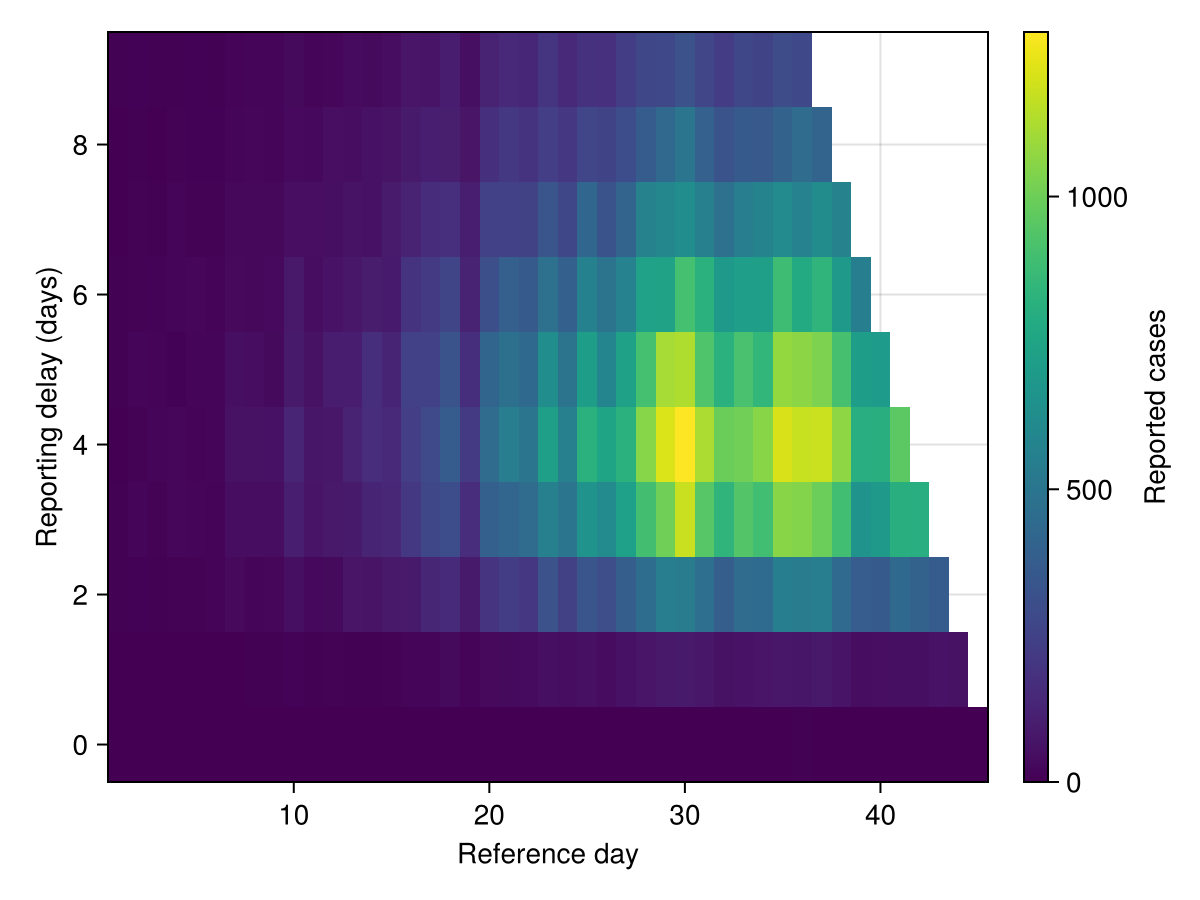
The same truncation reads as a shortfall in the tail when the observed-so-far row-sums are drawn against the eventual totals.
comp_df = DataFrame(
    reference = repeat(1:n, 2),
    count = vcat(eventual, observed_so_far),
    series = repeat(["eventual total", "observed so far"], inner = n))

draw(data(comp_df) * mapping(:reference, :count, color = :series) *
     visual(Lines); axis = (xlabel = "Reference day", ylabel = "Cases"))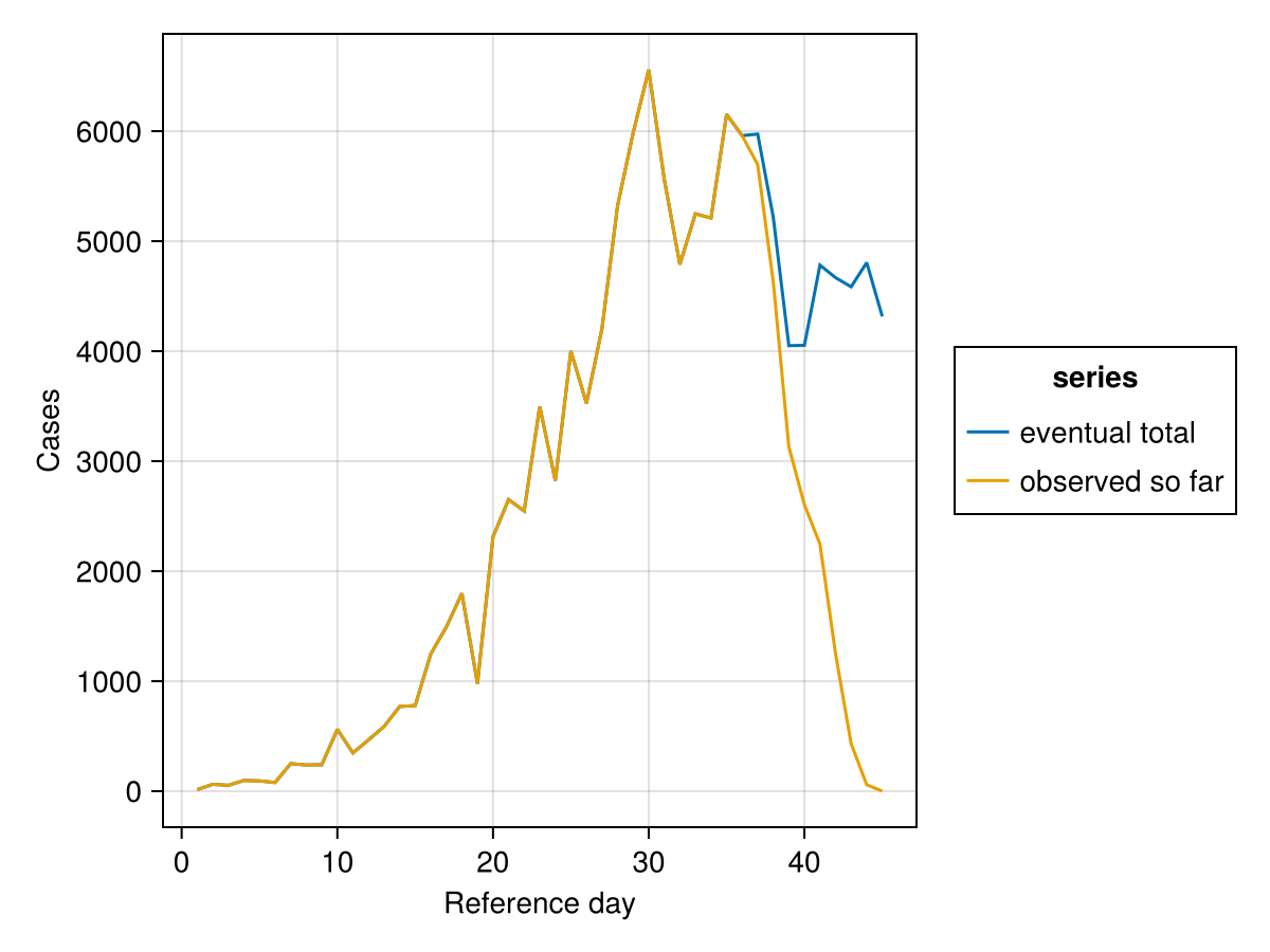
Three fits
We fit the plain renewal model three ways with NUTS, drawing two chains with 1000 warmup iterations each so the cross-chain RightTruncate applies the marginal correction to the same observed-so-far totals. ReportTriangle applies the joint correction to the reporting triangle, built through the shared define_y_t hook.
naive_model = IDModel(renewal, error)
naive_post = as_turing_model(naive_model, observed_so_far, n)
naive_chain = sample(
    naive_post, NUTS(1000, 0.95; adtype = adt), MCMCThreads(), 250, 2;
    progress = false)

rt_obs = RightTruncate(error, ReportingCDF(reporting_delay; D = 10))
rt_model = IDModel(renewal, rt_obs)
rt_post = as_turing_model(rt_model, observed_so_far, n)
rt_chain = sample(
    rt_post, NUTS(1000, 0.95; adtype = adt), MCMCThreads(), 250, 2;
    progress = false)

tri_obs = ReportTriangle(error, delay_pmf)
tri_data = define_y_t(tri_obs, reported_triangle, eventual)
tri_model = IDModel(renewal, tri_obs)
tri_post = as_turing_model(tri_model, tri_data, n)
tri_chain = sample(
    tri_post, NUTS(1000, 0.95; adtype = adt), MCMCThreads(), 250, 2;
    progress = false)
┌ Info: Found initial step size
└ ϵ = 0.00625
┌ Info: Found initial step size
└ ϵ = 0.0125
┌ Info: Found initial step size
└ ϵ = 0.0125
┌ Info: Found initial step size
└ ϵ = 0.025
┌ Warning: There were 2 divergent transitions. Consider reparameterising your model or using a smaller step size. For adaptive samplers such as NUTS and HMCDA, consider increasing `target_accept`.
└ @ Turing.Inference ~/.julia/packages/Turing/WteH7/src/mcmc/hmc.jl:483
┌ Warning: There were 2 divergent transitions. Consider reparameterising your model or using a smaller step size. For adaptive samplers such as NUTS and HMCDA, consider increasing `target_accept`.
└ @ Turing.Inference ~/.julia/packages/Turing/WteH7/src/mcmc/hmc.jl:483
┌ Info: Found initial step size
└ ϵ = 0.00625
┌ Info: Found initial step size
└ ϵ = 0.003125As a reference we also fit the plain model to the complete (untruncated) series, what the analyst would eventually see.
complete_post = as_turing_model(naive_model, eventual, n)
complete_chain = sample(
    complete_post, NUTS(1000, 0.95; adtype = adt), MCMCThreads(), 250, 2;
    progress = false)
┌ Info: Found initial step size
└ ϵ = 0.0125
┌ Info: Found initial step size
└ ϵ = 0.0125
┌ Warning: There were 4 divergent transitions. Consider reparameterising your model or using a smaller step size. For adaptive samplers such as NUTS and HMCDA, consider increasing `target_accept`.
└ @ Turing.Inference ~/.julia/packages/Turing/WteH7/src/mcmc/hmc.jl:483
┌ Warning: There were 4 divergent transitions. Consider reparameterising your model or using a smaller step size. For adaptive samplers such as NUTS and HMCDA, consider increasing `target_accept`.
└ @ Turing.Inference ~/.julia/packages/Turing/WteH7/src/mcmc/hmc.jl:483Recent Rt
generated_observables. Averaging it over the most recent window shows the bias and its removal. Right-truncation biases the naive recent
using Statistics

function recent_Rt(post, chain; window = 7)
    gens = vec(generated_observables(post, nothing, chain).generated)
    Rt_mean = mean(exp.(g.Z_t) for g in gens)
    round(mean(Rt_mean[(end - window + 1):end]), digits = 2)
end

(complete = recent_Rt(complete_post, complete_chain),
    naive = recent_Rt(naive_post, naive_chain),
    right_truncate = recent_Rt(rt_post, rt_chain),
    report_triangle = recent_Rt(tri_post, tri_chain))
(complete = 0.91, naive = 0.3, right_truncate = 0.9, report_triangle = 0.88)Posterior prediction, nowcast, and Rt
Three views of the fits share the reference-day axis with the recent window shaded. The RightTruncate model's posterior-predictive observed-so-far, recovered with predict on the same model with the observations set to missing, against the data it was fit to.
ts = 1:n
Rt_complete = gen_bands(complete_post, complete_chain, g -> exp.(g.Z_t))
Rt_naive = gen_bands(naive_post, naive_chain, g -> exp.(g.Z_t))
Rt_rt = gen_bands(rt_post, rt_chain, g -> exp.(g.Z_t))
Rt_tri = gen_bands(tri_post, tri_chain, g -> exp.(g.Z_t))

now_rt = gen_bands(rt_post, rt_chain, g -> g.I_t)
now_tri = gen_bands(tri_post, tri_chain, g -> g.I_t)

rt_pred = predict(as_turing_model(rt_model, fill(missing, n), n), rt_chain)
yt = predictive_bands(rt_pred, n)

fig = Figure(; size = (780, 820))
ax1 = Axis(fig[1, 1]; ylabel = "Reproduction number Rₜ")
vspan!(ax1, n - 6, n; color = (:grey, 0.15))
ci_ribbon!(ax1, ts, Rt_complete; color = :black, label = "complete (reference)")
ci_ribbon!(ax1, ts, Rt_naive; color = :crimson, label = "naive")
ci_ribbon!(ax1, ts, Rt_rt; color = :seagreen, label = "right-truncate")
ci_ribbon!(ax1, ts, Rt_tri; color = :steelblue, label = "report-triangle")
hlines!(ax1, [1.0]; color = :grey, linestyle = :dash)
axislegend(ax1; position = :lb, nbanks = 2)

ax2 = Axis(fig[2, 1]; ylabel = "Eventual cases (nowcast)")
vspan!(ax2, n - 6, n; color = (:grey, 0.15))
ci_ribbon!(ax2, ts, now_rt; color = :seagreen, label = "right-truncate")
ci_ribbon!(ax2, ts, now_tri; color = :steelblue, label = "report-triangle")
lines!(ax2, ts, Float64.(eventual); color = :black, linewidth = 2,
    label = "true eventual")
scatter!(ax2, ts, observed_so_far; color = :grey, markersize = 6,
    label = "observed so far")
axislegend(ax2; position = :lt)

ax3 = Axis(fig[3, 1]; xlabel = "Reference day", ylabel = "Observed-so-far")
vspan!(ax3, n - 6, n; color = (:grey, 0.15))
ci_ribbon!(ax3, ts, yt; color = :teal, label = "posterior predictive")
scatter!(ax3, ts, observed_so_far; color = :black, markersize = 6,
    label = "observed")
axislegend(ax3; position = :lt)
fig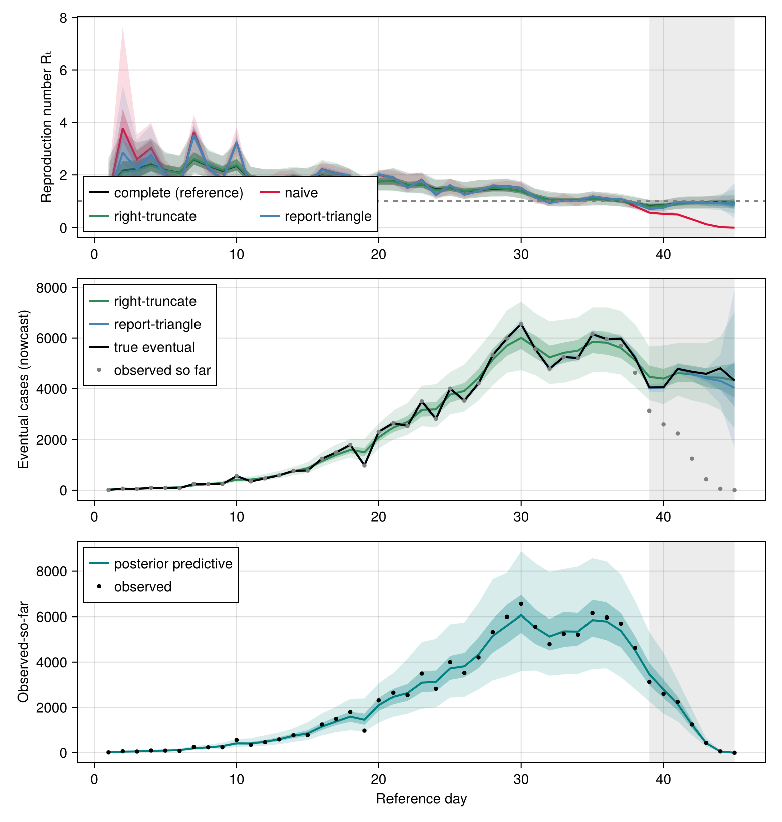
In the shaded recent window the naive RightTruncate fit reproduces the observed-so-far series it saw.
Shared parameters
Neither correction touches the renewal process, so both recover the same shared parameters, the autoregressive damping damp_AR[1]), the innovation scale std), the observation overdispersion (cluster_factor) and the initial infections (init_incidence). sample returns a FlexiChains chain that summarystats summarises directly, giving point estimates and their uncertainty alongside the effective sample size and
using MCMCChains
summarystats(tri_chain)╭─FlexiSummary (9 statistics) ─────────────────────────────────────────────────╮
│ iter collapsed │
│ chain collapsed │
│ ↓ stat = [mean, std, mcse, ess_bulk, ess_tail, rhat, q5, q50, q95] │
│ │
│ Parameters (50) ── AbstractPPL.VarName │
│ Float64 ar_init[1], damp_AR, ρ, std, ϵ_t[1], ϵ_t[2], ϵ_t[3], ϵ_t[4], │
│ ϵ_t[5], ϵ_t[6], ϵ_t[7], ϵ_t[8], ϵ_t[9], ϵ_t[10], ϵ_t[11], ϵ_t[12], │
│ ϵ_t[13], ϵ_t[14], ϵ_t[15], ϵ_t[16], ϵ_t[17], ϵ_t[18], ϵ_t[19], │
│ ϵ_t[20], ϵ_t[21], ϵ_t[22], ϵ_t[23], ϵ_t[24], ϵ_t[25], ϵ_t[26], │
│ ϵ_t[27], ϵ_t[28], ϵ_t[29], ϵ_t[30], ϵ_t[31], ϵ_t[32], ϵ_t[33], │
│ ϵ_t[34], ϵ_t[35], ϵ_t[36], ϵ_t[37], ϵ_t[38], ϵ_t[39], ϵ_t[40], │
│ ϵ_t[41], ϵ_t[42], ϵ_t[43], ϵ_t[44], init_incidence, │
│ cluster_factor │
│ │
│ Extras (14) │
│ Float64 n_steps, is_accept, acceptance_rate, log_density, │
│ hamiltonian_energy, hamiltonian_energy_error, │
│ max_hamiltonian_energy_error, tree_depth, numerical_error, │
│ step_size, nom_step_size, logprior, loglikelihood, logjoint │
│ │
│ Summary │
│ param mean std mcse ess_bulk ess_tail rhat … │
│ ar_init[1] 0.1094 0.2945 0.0408 52.2869 124.4964 1.0105 … │
│ damp_AR 0.7852 0.0454 0.0128 13.3155 24.3737 1.1138 … │
│ ρ 0.7852 0.0454 0.0128 13.3155 24.3737 1.1138 … │
│ std 0.3148 0.0294 0.0077 14.9360 67.8589 1.0253 … │
│ ϵ_t[1] 3.0095 0.7620 0.1198 40.0006 75.7999 1.0003 … │
│ ϵ_t[2] -0.0854 0.6565 0.0971 45.4632 96.2948 1.0369 … │
│ ϵ_t[3] 1.2589 0.5016 0.0600 69.4697 128.1853 1.0092 … │
│ ϵ_t[4] -0.3527 0.4472 0.0696 41.2500 76.7839 1.0066 … │
│ ϵ_t[5] -0.3993 0.4332 0.0531 64.7339 179.1219 1.0129 … │
│ ϵ_t[6] 2.9733 0.4296 0.0688 39.1950 143.0691 1.0245 … │
│ ϵ_t[7] -0.5177 0.3978 0.0539 51.2277 72.1730 1.0111 … │
│ ϵ_t[8] -0.2313 0.3078 0.0339 82.2107 81.0039 1.0292 … │
│ ϵ_t[9] 2.3240 0.3148 0.0737 18.5211 157.8487 1.0658 … │
│ ϵ_t[10] -1.8655 0.3171 0.0550 34.6663 54.1900 1.0059 … │
│ ϵ_t[11] 0.6812 0.2159 0.0285 57.5742 153.4576 1.0471 … │
│ ϵ_t[12] 0.5739 0.2281 0.0319 52.9186 120.1233 0.9998 … │
│ ϵ_t[13] 0.7078 0.2335 0.0378 43.3391 45.8115 1.0390 … │
│ ϵ_t[14] -0.1104 0.1889 0.0298 41.8889 90.3873 1.0186 … │
│ ϵ_t[15] 1.3140 0.1868 0.0346 30.0329 93.7628 1.0515 … │
│ ϵ_t[16] 0.3393 0.1895 0.0438 18.4541 59.8187 1.0922 … │
│ ϵ_t[17] 0.3378 0.1608 0.0228 50.4305 80.1942 1.0394 … │
│ ϵ_t[18] -2.1164 0.2550 0.0642 16.0929 53.0730 1.0231 … │
│ ϵ_t[19] 2.5823 0.2577 0.0621 17.5352 110.8657 1.0141 … │
│ ϵ_t[20] 0.2819 0.1482 0.0302 24.1805 59.5399 1.0626 … │
│ ϵ_t[21] -0.3218 0.1446 0.0327 21.7816 36.0683 1.0375 … │
│ ϵ_t[22] 0.8772 0.1222 0.0449 7.6203 102.9531 1.1161 … │
│ ϵ_t[23] -0.8305 0.1465 0.0319 21.8458 50.6233 1.0300 … │
│ ϵ_t[24] 1.0067 0.1243 0.0469 7.1362 56.7148 1.1247 … │
│ ϵ_t[25] -0.5098 0.1221 0.0265 23.1316 29.7655 1.0105 … │
│ ϵ_t[26] 0.4902 0.0863 0.0153 32.4077 150.9689 1.0301 … │
│ ϵ_t[27] 0.6823 0.1030 0.0309 11.9393 74.7083 1.0981 … │
│ ϵ_t[28] 0.2721 0.0906 0.0188 24.6573 152.8915 1.0589 … │
│ ϵ_t[29] 0.1741 0.0951 0.0186 26.4076 67.0805 1.0571 … │
│ ϵ_t[30] -0.6289 0.1062 0.0225 23.7375 56.1426 1.0149 … │
│ ϵ_t[31] -0.5608 0.0910 0.0185 23.7597 126.1150 1.0026 … │
│ ϵ_t[32] 0.2604 0.0706 0.0107 43.7884 98.2595 1.0053 … │
│ ϵ_t[33] -0.0363 0.0686 0.0081 72.0363 89.3700 1.0102 … │
│ ϵ_t[34] 0.5202 0.0787 0.0138 32.7071 49.9605 1.0157 … │
│ ϵ_t[35] -0.1255 0.0737 0.0153 28.0702 41.9504 1.0410 … │
│ ϵ_t[36] 0.0078 0.0685 0.0082 71.6017 100.6130 1.0141 … │
│ ϵ_t[37] -0.4456 0.0823 0.0170 24.8957 51.3290 1.0079 … │
│ ϵ_t[38] -0.8750 0.1086 0.0175 38.5713 108.3424 1.0120 … │
│ ϵ_t[39] -0.0173 0.1022 0.0264 17.0288 94.1350 1.1036 … │
│ ϵ_t[40] 0.5459 0.1260 0.0287 20.0922 79.5522 1.0100 … │
│ ϵ_t[41] -0.0917 0.1271 0.0173 57.0024 47.7412 1.0263 … │
│ ϵ_t[42] -0.1277 0.1777 0.0228 62.3276 124.5383 1.0034 … │
│ ϵ_t[43] -0.0793 0.4144 0.0452 84.4568 226.8501 1.0014 … │
│ ϵ_t[44] -0.1911 1.0513 0.1074 104.4454 88.0014 1.0024 … │
│ init_incide… 2.9540 0.2561 0.0408 39.9272 75.0883 1.0092 … │
│ cluster_fac… 0.0101 0.0062 0.0005 126.0732 99.9814 1.0000 … │
╰──────────────────────────────────────────────────────────────────────────────╯Prior versus posterior
Sampling the reporting-triangle model with Prior and overlaying it on the posterior with PairPlots.jl confirms the joint correction still identifies the shared parameters from the thinned triangle.
using PairPlots

prior_chain = sample(tri_post, Prior(), 1000; progress = false)
pp_keys = [@varname(damp_AR), @varname(std),
    @varname(cluster_factor), @varname(init_incidence)]
pairplot(
    PairPlots.Series(tri_chain[pp_keys]; label = "posterior"),
    PairPlots.Series(prior_chain[pp_keys]; label = "prior"))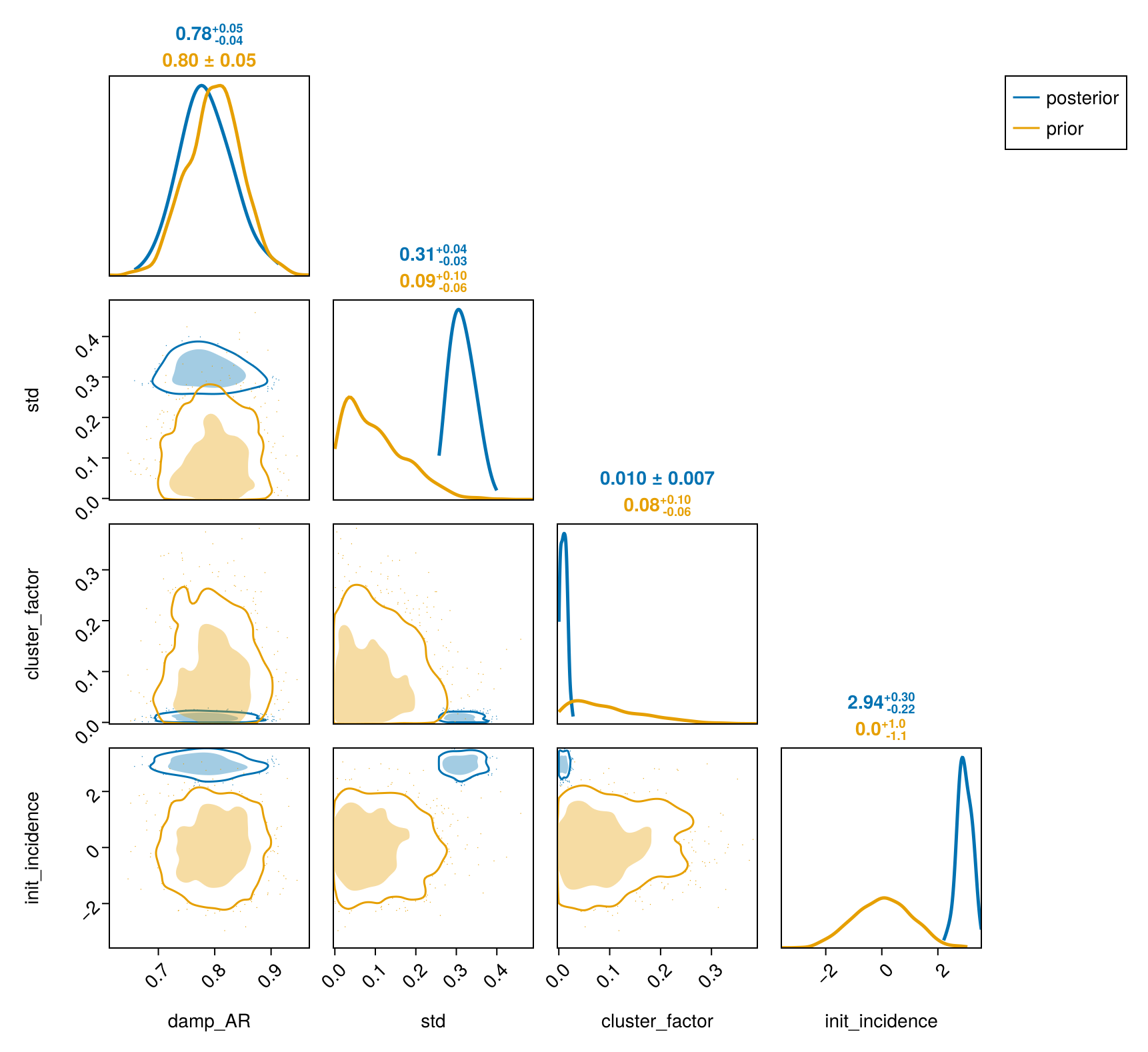
References
- S. Abbott, J. Hellewell, R. N. Thompson, K. Sherratt, H. P. Gibbs, N. I. Bosse, J. D. Munday, S. Meakin, E. L. Doughty, J. Y. Chun and others. Estimating the time-varying reproduction number of SARS-CoV-2 using national and subnational case counts. Wellcome Open Research 5, 112 (2020).