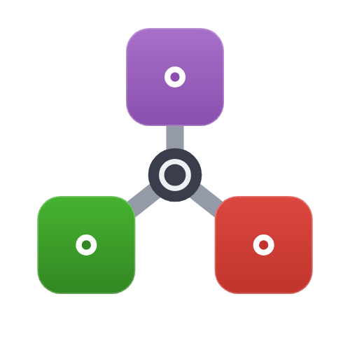
Multiple observation streams: cases, deaths, and strata
Real-time surveillance rarely watches an epidemic through a single lens. The same infections surface as reported cases, hospital admissions, deaths, and often each of these split by age, region, or variant. These streams share one underlying infection process but differ in their reporting delay, ascertainment, and noise [4]. Fitting them jointly — one infection trajectory, several observation streams — propagates uncertainty correctly and lets a sparse stream (deaths) borrow strength from a dense one (cases).
This tutorial uses one construct, Split, for every multi-stream shape. Split observes the expected series arriving at the point where it sits in the pipeline through several named streams, so where you place it chooses the composition:
parallel — placed high, on infections: every stream observes the same
(cases and deaths each a delayed, ascertained fraction of ); cascade — placed low, after a shared layer: a later stream is observed downstream of an earlier one (deaths as a delayed fraction of the expected reported cases);
strata — one stream per data-defined group (an age band).
How Split threads streams
Every observation model in the package returns the uniform pair (; y_t, expected): the sampled observations y_t and the pre-error expected series the error was scored against. Exposing expected is what lets Split do all three shapes with one mechanism. Split feeds each stream the expected series reaching it, and — because Split is itself an observation model — a shared modifier can run before it. Split((cases = …, deaths = …)) on its own splits infections (parallel), while LatentDelay(Split((cases = …, deaths = …)), pmf) applies a common delay first and then splits, so a stream nested inside another stream's pipeline sits downstream of it (cascade).
The threaded quantity is the expected, not the realised, series
A downstream stream reads its upstream stream's expected (pre-error) series, never its realised, sampled counts. So a cascade threads the mean reported cases into deaths, not a noisy draw. The case where an observation depends on another stream's realised (error-corrupted) observation — feeding sampled cases, not expected cases, into deaths — is not covered here and is out of scope for now.
Split also prefixes each stream's sampled variables with the stream name automatically, so the streams stay distinct without any manual prefix layer.
Parallel: cases and deaths from shared infections
We drive the streams with a renewal infection process, exactly as in the renewal tutorial, and observe it through two pipelines. Cases are a short-delay, high-ascertainment negative-binomial stream. Deaths are a long-delay stream whose ascertainment — the infection-fatality ratio — is itself estimated: each stream is a full observation model, so its ascertainment can be a fixed fraction or, as here, a latent Intercept model with a prior.
using ComposableTuringIDModels, Distributions, Random, Turing, Mooncake
using ADTypes: AutoMooncake
Random.seed!(1234)

latent = AR(
    damp = [truncated(Normal(0.8, 0.05), 0, 1),
        truncated(Normal(0.1, 0.05), 0, 1)],
    init = [Normal(0.0, 0.2), Normal(0.0, 0.2)],
    ϵ_t = HierarchicalNormal(std = HalfNormal(0.1)))
renewal = Renewal(; generation_time = Gamma(6.5, 0.62),
    rt = latent, initialisation = Normal(log(100.0), 0.1))

cases = LatentDelay(
    Ascertainment(NegativeBinomialError(cluster_factor = HalfNormal(0.1)),
        FixedIntercept(log(0.6))),                     # ~60% case ascertainment
    LogNormal(1.6, 0.5))                                # short infection→report delay
deaths = LatentDelay(
    Ascertainment(NegativeBinomialError(cluster_factor = HalfNormal(0.1)),
        Intercept(Normal(log(0.015), 0.25))),          # estimated ~1.5% IFR
    LogNormal(2.8, 0.4))                                # long infection→death delay

parallel = Split((cases = cases, deaths = deaths))
Split
├─ cases: LatentDelay
│ └─ model: Ascertainment
│ ├─ model: NegativeBinomialError
│ └─ latent: PrefixLatentModel
│ └─ model: FixedIntercept
└─ deaths: LatentDelay
└─ model: Ascertainment
├─ model: NegativeBinomialError
└─ latent: PrefixLatentModel
└─ model: InterceptThe composed model assembles the renewal infection process and the two-stream observation model exactly like a single-stream study.
model = IDModel(renewal, parallel)IDModel
├─ infection: Renewal
│ └─ rt: AR
│ └─ ϵ_t: HierarchicalNormal
└─ observation: Split
├─ cases: LatentDelay
│ └─ model: Ascertainment
│ ├─ model: NegativeBinomialError
│ └─ latent: PrefixLatentModel
│ └─ model: FixedIntercept
└─ deaths: LatentDelay
└─ model: Ascertainment
├─ model: NegativeBinomialError
└─ latent: PrefixLatentModel
└─ model: InterceptPassing missing data simulates a synthetic outbreak. The per-stream data contract is a NamedTuple keyed by stream name, and the returned generated_y_t is a NamedTuple of the two simulated series.
n = 70
sim = as_turing_model(model, (cases = missing, deaths = missing), n)()
y = sim.generated_y_t
(total_cases = sum(skipmissing(y.cases)), total_deaths = sum(skipmissing(y.deaths)))
(total_cases = 6576, total_deaths = 82)Fitting conditions on both streams at once. We draw a full chain with NUTS, matching the other tutorials, and differentiate with Mooncake, the recommended backend for this package (see Automatic differentiation backend).
ydata = (cases = y.cases, deaths = y.deaths)
posterior = as_turing_model(model, ydata, n)
chain = sample(
    posterior, NUTS(0.95; adtype = AutoMooncake(; config = nothing)),
    MCMCThreads(), 250, 2; progress = false)
┌ Info: Found initial step size
└ ϵ = 0.025
┌ Info: Found initial step size
└ ϵ = 0.00625
┌ Warning: There were 11 divergent transitions. Consider reparameterising your model or using a smaller step size. For adaptive samplers such as NUTS and HMCDA, consider increasing `target_accept`.
└ @ Turing.Inference ~/.julia/packages/Turing/WteH7/src/mcmc/hmc.jl:483
┌ Warning: There were 5 divergent transitions. Consider reparameterising your model or using a smaller step size. For adaptive samplers such as NUTS and HMCDA, consider increasing `target_accept`.
└ @ Turing.Inference ~/.julia/packages/Turing/WteH7/src/mcmc/hmc.jl:483
┌ Warning: There were 16 divergent transitions. Consider reparameterising your model or using a smaller step size. For adaptive samplers such as NUTS and HMCDA, consider increasing `target_accept`.
└ @ Turing.Inference ~/.julia/packages/Turing/WteH7/src/mcmc/hmc.jl:483The two streams keep their own overdispersion parameters — Split prefixes them cases.cluster_factor and deaths.cluster_factor — while sharing the one infection trajectory, and the deaths stream's estimated IFR intercept (deaths.Ascertainment.intercept) is recovered alongside them. The dense case stream pins the shared
using MCMCChains
summarystats(chain)╭─FlexiSummary (9 statistics) ─────────────────────────────────────────────────╮
│ iter collapsed │
│ chain collapsed │
│ ↓ stat = [mean, std, mcse, ess_bulk, ess_tail, rhat, q5, q50, q95] │
│ │
│ Parameters (77) ── AbstractPPL.VarName │
│ Float64 ar_init[1], ar_init[2], damp_AR[1], damp_AR[2], std, ϵ_t[1], │
│ ϵ_t[2], ϵ_t[3], ϵ_t[4], ϵ_t[5], ϵ_t[6], ϵ_t[7], ϵ_t[8], ϵ_t[9], │
│ ϵ_t[10], ϵ_t[11], ϵ_t[12], ϵ_t[13], ϵ_t[14], ϵ_t[15], ϵ_t[16], │
│ ϵ_t[17], ϵ_t[18], ϵ_t[19], ϵ_t[20], ϵ_t[21], ϵ_t[22], ϵ_t[23], │
│ ϵ_t[24], ϵ_t[25], ϵ_t[26], ϵ_t[27], ϵ_t[28], ϵ_t[29], ϵ_t[30], │
│ ϵ_t[31], ϵ_t[32], ϵ_t[33], ϵ_t[34], ϵ_t[35], ϵ_t[36], ϵ_t[37], │
│ ϵ_t[38], ϵ_t[39], ϵ_t[40], ϵ_t[41], ϵ_t[42], ϵ_t[43], ϵ_t[44], │
│ ϵ_t[45], ϵ_t[46], ϵ_t[47], ϵ_t[48], ϵ_t[49], ϵ_t[50], ϵ_t[51], │
│ ϵ_t[52], ϵ_t[53], ϵ_t[54], ϵ_t[55], ϵ_t[56], ϵ_t[57], ϵ_t[58], │
│ ϵ_t[59], ϵ_t[60], ϵ_t[61], ϵ_t[62], ϵ_t[63], ϵ_t[64], ϵ_t[65], │
│ ϵ_t[66], ϵ_t[67], ϵ_t[68], init_incidence, cases.cluster_factor, │
│ deaths.Ascertainment.intercept, deaths.cluster_factor │
│ │
│ Extras (14) │
│ Float64 n_steps, is_accept, acceptance_rate, log_density, │
│ hamiltonian_energy, hamiltonian_energy_error, │
│ max_hamiltonian_energy_error, tree_depth, numerical_error, │
│ step_size, nom_step_size, logprior, loglikelihood, logjoint │
│ │
│ Summary │
│ param mean std mcse ess_bulk ess_tail rhat … │
│ ar_init[1] -0.0134 0.1977 0.0087 517.4269 292.1407 0.9980 … │
│ ar_init[2] 0.3000 0.1460 0.0061 562.7938 345.7154 0.9993 … │
│ damp_AR[1] 0.7901 0.0413 0.0021 388.1683 472.2365 0.9980 … │
│ damp_AR[2] 0.0881 0.0405 0.0019 401.4252 313.4341 0.9995 … │
│ std 0.0683 0.0313 0.0018 272.4745 291.9637 0.9998 … │
│ ϵ_t[1] 0.4855 0.9823 0.0444 481.4656 312.6769 0.9997 … │
│ ϵ_t[2] 0.3797 1.0069 0.0412 609.6156 321.5575 1.0005 … │
│ ϵ_t[3] 0.4112 0.9692 0.0368 696.4376 236.7163 1.0033 … │
│ ϵ_t[4] 0.3098 0.9562 0.0410 539.8658 183.5606 1.0074 … │
│ ϵ_t[5] 0.3122 0.9783 0.0359 740.6972 346.5598 1.0006 … │
│ ϵ_t[6] 0.1987 0.9615 0.0373 647.0263 343.7761 1.0012 … │
│ ϵ_t[7] 0.2094 0.9767 0.0376 674.7942 264.6674 0.9996 … │
│ ϵ_t[8] 0.0762 0.9708 0.0390 628.1686 273.8790 1.0035 … │
│ ϵ_t[9] 0.0081 0.9721 0.0418 538.1227 309.5746 1.0133 … │
│ ϵ_t[10] -0.0346 0.9299 0.0343 737.0287 296.7789 0.9990 … │
│ ϵ_t[11] -0.0568 0.9680 0.0415 542.3656 321.9191 1.0090 … │
│ ϵ_t[12] -0.1395 0.9674 0.0428 506.4988 328.3563 0.9984 … │
│ ϵ_t[13] -0.1573 0.9817 0.0357 767.8499 278.4443 1.0044 … │
│ ϵ_t[14] -0.1081 0.9288 0.0390 569.4577 284.6925 1.0042 … │
│ ϵ_t[15] -0.1584 1.0621 0.0399 718.8924 281.7445 1.0001 … │
│ ϵ_t[16] -0.1533 0.8792 0.0320 756.2154 449.1737 0.9987 … │
│ ϵ_t[17] -0.0997 0.9050 0.0352 644.7473 385.8729 0.9991 … │
│ ϵ_t[18] -0.1431 0.8485 0.0320 710.0472 286.7976 1.0047 … │
│ ϵ_t[19] -0.1950 0.9851 0.0356 784.6508 289.5902 1.0037 … │
│ ϵ_t[20] -0.0574 0.9913 0.0376 691.5219 382.0824 0.9980 … │
│ ϵ_t[21] -0.1900 0.9194 0.0358 675.6951 350.9691 1.0028 … │
│ ϵ_t[22] -0.2373 0.9446 0.0340 773.6037 332.4821 0.9989 … │
│ ϵ_t[23] -0.3198 0.9005 0.0334 714.9404 456.9490 0.9994 … │
│ ϵ_t[24] -0.3829 0.9644 0.0364 702.6158 375.4466 1.0123 … │
│ ϵ_t[25] -0.2545 0.9559 0.0385 626.0014 273.2563 1.0002 … │
│ ϵ_t[26] -0.2121 0.8898 0.0414 491.5460 293.4143 0.9991 … │
│ ϵ_t[27] -0.2197 1.0004 0.0443 538.0812 235.3372 1.0009 … │
│ ϵ_t[28] -0.3481 0.8894 0.0348 668.4585 293.4143 1.0249 … │
│ ϵ_t[29] -0.3342 1.0035 0.0371 733.8012 369.1484 1.0016 … │
│ ϵ_t[30] -0.3521 1.0158 0.0385 696.9638 328.5913 1.0009 … │
│ ϵ_t[31] -0.3600 0.8785 0.0374 573.5196 425.5089 1.0206 … │
│ ϵ_t[32] -0.3837 0.9353 0.0331 825.3964 344.5669 1.0008 … │
│ ϵ_t[33] -0.3660 0.9410 0.0355 696.7572 345.8745 0.9998 … │
│ ϵ_t[34] -0.3435 1.0130 0.0433 563.7248 336.3859 1.0052 … │
│ ϵ_t[35] -0.4461 0.9726 0.0348 783.7977 317.8898 1.0050 … │
│ ϵ_t[36] -0.3517 0.8870 0.0351 633.2882 397.1590 0.9996 … │
│ ϵ_t[37] -0.3282 0.9393 0.0385 565.6660 349.1117 0.9981 … │
│ ϵ_t[38] -0.1420 0.9615 0.0340 809.1725 491.3931 0.9989 … │
│ ϵ_t[39] -0.0167 0.9691 0.0367 687.4058 349.8661 0.9997 … │
│ ϵ_t[40] 0.0838 0.9207 0.0363 626.9669 265.2131 1.0141 … │
│ ϵ_t[41] 0.1620 0.9682 0.0350 762.8732 288.2856 0.9994 … │
│ ϵ_t[42] 0.3361 0.9385 0.0338 770.9451 378.9851 1.0004 … │
│ ϵ_t[43] 0.4005 0.9463 0.0337 804.5095 283.5594 0.9986 … │
│ ϵ_t[44] 0.5345 0.8989 0.0373 572.2967 304.4086 0.9984 … │
│ ϵ_t[45] 0.3982 0.9432 0.0428 499.9170 236.0082 1.0009 … │
│ ϵ_t[46] 0.1936 1.0212 0.0384 717.3304 342.9982 0.9985 … │
│ ϵ_t[47] 0.2416 1.0199 0.0396 667.7880 335.4155 1.0280 … │
│ ϵ_t[48] 0.2587 0.9714 0.0380 661.8740 390.9766 0.9993 … │
│ ϵ_t[49] 0.3670 0.9982 0.0400 629.2939 321.5575 1.0065 … │
│ ϵ_t[50] 0.3678 0.9605 0.0391 603.1109 453.7388 0.9984 … │
│ ϵ_t[51] 0.2832 0.9748 0.0376 670.6878 400.7875 1.0000 … │
│ ϵ_t[52] 0.2958 0.9516 0.0293 1038.4850 472.2365 0.9995 … │
│ ϵ_t[53] 0.1534 1.0326 0.0403 704.9446 148.2672 0.9982 … │
│ ϵ_t[54] 0.0287 0.9415 0.0404 541.7738 319.1300 1.0053 … │
│ ϵ_t[55] -0.0275 0.9828 0.0383 655.7541 408.5154 1.0028 … │
│ ϵ_t[56] -0.0404 1.0665 0.0451 563.9972 301.9859 1.0074 … │
│ ϵ_t[57] -0.0530 0.9900 0.0365 720.4855 408.1275 0.9997 … │
│ ϵ_t[58] 0.0165 0.9874 0.0318 972.5631 438.5675 1.0041 … │
│ ϵ_t[59] 0.0831 0.9473 0.0276 1196.6038 368.7272 0.9988 … │
│ ϵ_t[60] 0.2274 0.9478 0.0358 693.1988 326.9978 1.0027 … │
│ ϵ_t[61] 0.2705 0.9116 0.0426 458.0932 279.9381 1.0000 … │
│ ϵ_t[62] 0.2296 0.9998 0.0413 586.6932 397.1099 0.9984 … │
│ ϵ_t[63] 0.1009 0.9989 0.0377 710.0976 463.3332 0.9999 … │
│ ϵ_t[64] -0.0042 0.9863 0.0417 565.9914 374.3784 0.9996 … │
│ ϵ_t[65] -0.0296 0.9673 0.0404 571.0509 247.6054 1.0046 … │
│ ϵ_t[66] 0.0042 1.0804 0.0480 497.5813 287.6045 0.9992 … │
│ ϵ_t[67] 0.0351 0.9498 0.0356 701.9941 388.2477 0.9997 … │
│ ϵ_t[68] -0.0406 0.9824 0.0367 717.0431 429.7968 0.9992 … │
│ init_incide… 4.6598 0.0925 0.0039 576.7949 459.6035 0.9982 … │
│ cases.clust… 0.0948 0.0203 0.0010 395.0110 262.2740 1.0016 … │
│ deaths.Asce… -4.1922 0.1120 0.0051 476.0261 302.7490 1.0006 … │
│ deaths.clus… 0.1059 0.0776 0.0029 535.0296 238.1595 0.9997 … │
╰──────────────────────────────────────────────────────────────────────────────╯Cascade: deaths downstream of reported cases
In the parallel model, cases and deaths both branch off infections, so a reporting artefact in the case series (a weekend dip, an ascertainment change) does not touch deaths. Sometimes we want the opposite: deaths modelled as a delayed fraction of the reported cases, so whatever is reflected in cases propagates into deaths. That is a cascade Split placed lower in the stack. Share the infection→case-report delay, then split: the cases stream applies its error to the delayed expectation, and the deaths stream sits downstream, delayed again by the case-report→death interval and scaled by the fatality fraction.
cascade = LatentDelay(                                   # infection→case delay
    Split((
        cases = NegativeBinomialError(cluster_factor = HalfNormal(0.1)),
        deaths = LatentDelay(                            # case→death delay
            Ascertainment(NegativeBinomialError(cluster_factor = HalfNormal(0.1)),
                FixedIntercept(log(0.02))),
            LogNormal(2.2, 0.3)))),
    LogNormal(1.6, 0.5))
cascade_model = IDModel(renewal, cascade)
cas = as_turing_model(cascade_model, (cases = missing, deaths = missing), n)()
(generated_y_t = (cases = Union{Missing, Int64}[270, 218, 297, 216, 337, 350, 349, 317, 345, 235 … 18, 24, 42, 36, 27, 32, 26, 28, 15, 16], deaths = Union{Missing, Int64}[missing, missing, missing, missing, missing, missing, missing, missing, missing, missing … 2, 0, 1, 1, 2, 1, 1, 0, 0, 0]), expected_y_t = (cases = [227.09297655006515, 243.34766824296463, 261.4816875378536, 278.27562743143085, 290.96278567072767, 301.28182061015445, 312.3983423411687, 324.84589430964934, 335.202679731171, 339.20058769222027 … 31.186316265782253, 28.694989824511705, 26.443695240615767, 24.485114690631935, 22.78252119789874, 21.169716185551703, 19.462217764470928, 17.66258532039228, 15.938218082601624, 14.34144459929579], deaths = [6.438898577278827, 6.5269959308405525, 6.567662962367721, 6.564000144659306, 6.517047629226356, 6.424169592255847, 6.280901953934637, 6.084810397911528, 5.83805796271519, 5.547591893051596 … 1.1520649516076364, 1.0772106846356608, 1.0106802434475666, 0.9503586772567195, 0.8943779493996301, 0.8411996384132008, 0.7896930783313534, 0.7392927313360437, 0.6900632656439989, 0.6424963952669404]), I_t = [124.82023240024644, 118.78877067901828, 125.14877354497487, 134.7185804215374, 158.58527604659736, 156.77778466087594, 176.86934435498142, 184.48537949475954, 201.74499799634336, 237.88281397858523 … 20.165685555311363, 18.84224824466163, 17.72302898875249, 15.751613393207492, 12.275154235021288, 11.731027928240005, 10.62287226771338, 9.386131507924807, 7.465721130334034, 5.331369642723158], Z_t = [0.5312446389953557, 0.3423504104670212, 0.26194720091244966, 0.23095905875602335, 0.32222357859830564, 0.25145249562109956, 0.3032385726661695, 0.2704627134438929, 0.28597582344222056, 0.3785932527760605 … -0.30701422716001253, -0.28013584652799267, -0.2573887741920619, -0.3042302765638896, -0.4888920355466817, -0.4624106916544015, -0.4674184012263106, -0.47696013976741813, -0.5856294205914864, -0.8032070473681383])The Split sits after the shared case delay and before the error leaves, so the deaths stream's expected input is the delayed-and-ascertained expected cases, not the raw infections: it is both scaled by the fatality fraction and shortened by the case delay.
(cases_expected_length = length(cas.expected_y_t.cases),
    deaths_expected_length = length(cas.expected_y_t.deaths),
    deaths_are_a_fraction_of_cases =
        sum(cas.expected_y_t.deaths) < sum(cas.expected_y_t.cases))
(cases_expected_length = 55, deaths_expected_length = 38, deaths_are_a_fraction_of_cases = true)Strata: one stream per age band
A stratified stream — one observation series per age band, region, or variant — is again the same construct, here composed with the renewal infection process and observed through one named stream per band. Each band is a full observation model, so its delay and ascertainment can differ, and its parameters are namespaced by the band name.
strata_obs = Split((
    young = LatentDelay(
        Ascertainment(NegativeBinomialError(cluster_factor = HalfNormal(0.1)),
            FixedIntercept(log(0.7))), LogNormal(1.5, 0.4)),
    old = LatentDelay(
        Ascertainment(NegativeBinomialError(cluster_factor = HalfNormal(0.1)),
            FixedIntercept(log(0.4))), LogNormal(1.8, 0.4))))
strata_model = IDModel(renewal, strata_obs)
strata_sim = as_turing_model(
    strata_model, (young = missing, old = missing), n)().generated_y_t
map(s -> sum(skipmissing(s)), strata_sim)                # totals per band
(young = 2733, old = 1504)The streams above each observe the same infections. When the streams instead draw on a weighted mix of infections — one band, another band, and a summed total — the same Split carries an observation-strata × infection-strata weight matrix, and a single template model is replicated once per data stream. Split(template, W) projects the infection series reaching it through W, so it composes inside an IDModel like any other observation model: the infections come from the modelled process, not a hand-built series. One weight matrix covers the one-to-one (an identity map), many-to-one (an aggregation row summing infection strata into one stream), and many-to-many (a general matrix) infection → observation cases.
Here the renewal process supplies one infection stratum, and W maps it onto a young band, an old band, and their total:
W = reshape([0.7, 0.3, 1.0], 3, 1)                  # young, old, and their total
weighted = Split(LatentDelay(PoissonError(), LogNormal(1.6, 0.5)), W)
weighted_model = IDModel(renewal, weighted)
age = as_turing_model(
    weighted_model, (young = missing, old = missing, total = missing), n)()
map(s -> sum(skipmissing(s)), age.generated_y_t)         # simulated total per band
(young = 3718, old = 1619, total = 5585)The aggregate total stream sees the summed expected infections of both bands — its expected series is exactly young .+ old.
Here the single renewal process supplied one infection stratum, broadcast through W. When the strata are genuinely separate infection processes — several distinct regions, say, each with its own latent — swap the single infection model for CombineInfections: it draws each process independently and stacks the results into the same infection-strata × time matrix Split/StrataMap already expect, so IDModel(CombineInfections([...]), Split(template, W)) maps several distinct infection processes onto streams end-to-end. For one process carried across a strata axis instead, with partially pooled per-stratum deviations, see Stratify and Partial pooling across groups. It also composes with Renewal's mixing slot, see Coupled patch models.
References
- K. Sherratt, S. Abbott, S. R. Meakin, J. Hellewell, J. D. Munday, N. Bosse, M. Jit and S. Funk. Exploring surveillance data biases when estimating the reproduction number: with insights into subpopulation transmission of COVID-19 in England. Philosophical Transactions of the Royal Society B 376, 20200283 (2021).