Reporting delays and day-of-week effects

Real surveillance data is rarely a clean count of infections on the day they occur. Cases are reported after a delay — an incubation period followed by a reporting lag — and the number reported depends on the day of the week. Tools for real-time estimation such as those of Abbott et al. [3] build these features into the observation model so that the latent infection signal is estimated free of reporting artefacts.

This case study keeps the renewal infection core of the previous example but replaces the simple observation model with a layered one: infections are convolved through two delay distributions and then modulated by a day-of-week reporting pattern. It also shows the latent process as an ARIMA-style differenced process broadcast to a weekly timescale, and assembles everything with IDProblem. The model follows the configuration of the EpiNow2 package [3] and is fit to daily confirmed COVID-19 cases from Italy's first wave in 2020.

The model

where is the incubation-period pmf, the reporting-delay pmf, and a day-of-week reporting multiplier.

A weekly latent process

The latent process is an ARIMA(2,1,1): an AR/MA combination (arma) wrapped in a DiffLatentModel to difference it once. Differencing makes the level a random walk rather than mean-reverting, which suits a reproduction number that can drift.

using ComposableTuringIDModels, Distributions, Random, Turing, Mooncake
using ADTypes: AutoMooncake
Random.seed!(20240601)

arma21 = arma(
    init = [Normal(0, 0.2), Normal(0, 0.2)],
    damp = [truncated(Normal(0.1, 0.2), 0, 1), truncated(Normal(0.1, 0.05), 0, 1)],
    θ = [truncated(Normal(0.0, 0.2), -1, 1)],
    ϵ_t = HierarchicalNormal(std_prior = HalfNormal(0.1)))

arima211 = DiffLatentModel(; model = arma21, init_priors = [Normal(0.3, 0.3)])

broadcast_weekly makes the process piecewise-constant by week: a new value is drawn each week and held for seven days. This models as changing weekly rather than daily, which both regularises the estimate and cuts the number of latent parameters.

weekly_latent = broadcast_weekly(arima211)

The infection process

As before, a Renewal process driven by a discretised generation interval. Here we use a generation time. The weekly process built above is folded into the renewal model's rt slot.

renewal = Renewal(gen_distribution = Gamma(1.4, 1 / 0.38);
    rt = weekly_latent, initialisation_prior = Normal(log(1.0), 1.0))

A layered observation model

We start from the NegativeBinomialError link and build outward. ascertainment_dayofweek wraps it with a partially pooled day-of-week multiplier, so reporting can be systematically higher or lower on particular weekdays.

negbin = NegativeBinomialError(cluster_factor_prior = HalfNormal(0.1))
dayofweek_negbin = ascertainment_dayofweek(
    negbin; latent_model = HierarchicalNormal(std_prior = HalfNormal(1.0)))

LatentDelay convolves the expected observations with a delay distribution (discretised by double interval censoring). Two layers compose sequentially: an incubation period from infection to symptom onset, then a reporting delay from onset to report.

incubation = LogNormal(1.6, 0.42)   # infection -> symptom onset
reporting = LogNormal(0.58, 0.47)   # symptom onset -> report

observation = LatentDelay(LatentDelay(dayofweek_negbin, incubation), reporting)

That single observation object now carries, from the inside out: a negative binomial link, a day-of-week ascertainment modifier, an incubation-delay convolution, and a reporting-delay convolution — assembled entirely by composition.

The data

We fit the model to the daily confirmed COVID-19 cases from Italy's first wave (the example series shipped with the EpiNow2 package), stored with the docs.

using CSV, DataFrames
datapath = joinpath(pkgdir(ComposableTuringIDModels),
    "docs", "src", "case-studies", "data", "italy_data.csv")
italy = CSV.read(datapath, DataFrame)
n = 42
y_obs = italy.confirm[1:n]
(n = n, total_cases = sum(y_obs), from = italy.date[1], to = italy.date[n])

(n = 42, total_cases = 115239, from = Dates.Date("2020-02-22"), to = Dates.Date("2020-04-03"))

Assemble and fit

IDProblem ties the latent, infection, and observation models to a time span. Its as_turing_model method takes data as a named tuple with a y_t field (passing missing values would instead simulate from the prior).

problem = IDProblem(
    infection = renewal,
    observation_model = observation,
    tspan = (1, n))

Fitting conditions on the observed reports, differentiating with the recommended Mooncake backend (see Automatic differentiation backend). We draw two chains in parallel with MCMCThreads(), which gives a cross-chain :

posterior = as_turing_model(problem, (y_t = y_obs,))
chain = sample(
    posterior, NUTS(0.9; adtype = AutoMooncake(; config = nothing)),
    MCMCThreads(), 500, 2; progress = false)

┌ Warning: Only a single thread available: MCMC chains are not sampled in parallel
└ @ AbstractMCMC ~/.julia/packages/AbstractMCMC/C1aKp/src/sample.jl:544
┌ Info: Found initial step size
└   ϵ = 0.0125
┌ Info: Found initial step size
└   ϵ = 0.00078125

sample returns a FlexiChains chain, which summarystats summarises directly — no conversion step. The day-of-week scale (DayofWeek.std) and the negative-binomial overdispersion (cluster_factor) appear alongside the latent-process parameters:

using MCMCChains
summarystats(chain)

╭─FlexiSummary (9 statistics) ─────────────────────────────────────────────────╮
│   iter    collapsed                                                          │
│   chain   collapsed                                                          │
│ ↓ stat  = [mean, std, mcse, ess_bulk, ess_tail, rhat, q5, q50, q95]          │
│                                                                              │
│ Parameters (20) ── AbstractPPL.VarName                                       │
│  Float64  latent_init[1], ar_init[1], ar_init[2], damp_AR[1], damp_AR[2],    │
│           θ[1], std, ϵ_t[1], ϵ_t[2], ϵ_t[3], init_incidence, DayofWeek.std,  │
│           DayofWeek.ϵ_t[1], DayofWeek.ϵ_t[2], DayofWeek.ϵ_t[3],              │
│           DayofWeek.ϵ_t[4], DayofWeek.ϵ_t[5], DayofWeek.ϵ_t[6],              │
│           DayofWeek.ϵ_t[7], cluster_factor                                   │
│                                                                              │
│ Extras (14)                                                                  │
│  Float64  n_steps, is_accept, acceptance_rate, log_density,                  │
│           hamiltonian_energy, hamiltonian_energy_error,                      │
│           max_hamiltonian_energy_error, tree_depth, numerical_error,         │
│           step_size, nom_step_size, logprior, loglikelihood, logjoint        │
│                                                                              │
│ Summary                                                                      │
│          param     mean     std    mcse   ess_bulk  ess_tail    rhat  …      │
│   latent_init…   0.9197  0.1864  0.0105   316.6035  337.8295  1.0118  …      │
│     ar_init[1]  -0.1458  0.1837  0.0077   571.7815  565.7442  0.9998  …      │
│     ar_init[2]  -0.3597  0.1482  0.0071   440.8603  642.9180  1.0041  …      │
│     damp_AR[1]   0.3214  0.1651  0.0069   548.4288  431.7611  0.9991  …      │
│     damp_AR[2]   0.1118  0.0459  0.0026   317.3515  109.4817  1.0008  …      │
│           θ[1]   0.0285  0.1976  0.0056  1242.2276  742.9061  0.9993  …      │
│            std   0.1415  0.0756  0.0033   454.2904  295.9690  1.0007  …      │
│         ϵ_t[1]  -0.8925  0.7682  0.0320   608.5943  608.9184  1.0030  …      │
│         ϵ_t[2]  -0.7654  0.7502  0.0266   834.1756  676.1213  0.9996  …      │
│         ϵ_t[3]  -0.0501  0.9456  0.0263  1287.0323  727.6692  1.0127  …      │
│   init_incide…   4.1055  0.6600  0.0374   310.8287  239.9930  1.0100  …      │
│   DayofWeek.s…   0.1301  0.0737  0.0055   153.6420  282.3468  1.0022  …      │
│   DayofWeek.ϵ…   0.1083  0.6925  0.0250   741.1473  677.9194  0.9998  …      │
│   DayofWeek.ϵ…  -0.1865  0.6339  0.0223   814.0973  839.3778  0.9990  …      │
│   DayofWeek.ϵ…  -1.2675  0.7862  0.0323   625.5262  561.5812  1.0003  …      │
│   DayofWeek.ϵ…  -0.0857  0.6809  0.0218   984.4220  557.3453  0.9995  …      │
│   DayofWeek.ϵ…   0.4093  0.6844  0.0258   703.5654  628.7393  1.0003  …      │
│   DayofWeek.ϵ…   0.3116  0.7096  0.0234   938.1727  763.2700  0.9994  …      │
│   DayofWeek.ϵ…   0.7497  0.7334  0.0239   917.8499  663.1633  1.0007  …      │
│   cluster_fac…   0.1583  0.0279  0.0013   460.9402  634.3957  0.9998  …      │
╰──────────────────────────────────────────────────────────────────────────────╯

DayofWeek.std is the scale of the partially pooled weekday multipliers (its own block, prefixed because the ascertainment modifier introduces a named sub-process); cluster_factor is the negative-binomial overdispersion. The day-of-week effect, the two delay kernels, and the weekly reproduction number were all estimated jointly — and any of them can be swapped or removed by editing one line of the composition above.

Prior versus posterior

Sampling the same model with Prior gives a prior draw over the same parameters. Overlaying it on the posterior with PairPlots.jl — the FlexiChains extension turns each chain, subset to a few keys, into a PairPlots.Series — shows which parameters the six weeks of Italian data moved.

using CairoMakie, PairPlots

prior_chain = sample(posterior, Prior(), 1000; progress = false)
pp_keys = [@varname(damp_AR), @varname(θ), @varname(std),
    @varname(cluster_factor)]
pairplot(
    PairPlots.Series(chain[pp_keys]; label = "posterior"),
    PairPlots.Series(prior_chain[pp_keys]; label = "prior"))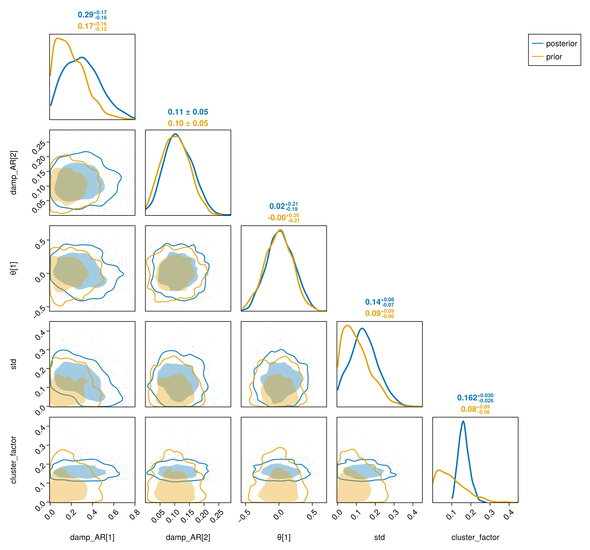

The innovation scale (std) and the negative-binomial overdispersion (cluster_factor) tighten under the data, while the autoregressive damping (damp_AR) and moving-average (θ) coefficients of the ARIMA process stay close to their weakly informative priors.

Posterior trajectories

  and the infections are generated quantities recovered per draw with generated_observables; the reports are scored element-wise, so their posterior-predictive distribution comes from predict on the model with the observations set to missing. Two small helpers reduce the per-draw trajectories to credible bands.

gens = vec(generated_observables(posterior, (y_t = y_obs,), chain).generated)
Rt = credible_bands(reduce(hcat, (exp.(g.Z_t) for g in gens)))

pred = predict(as_turing_model(problem, (y_t = fill(missing, n),)), chain)
yt = predictive_bands(pred, n)

fig = Figure(; size = (760, 620))
ax1 = Axis(fig[1, 1]; ylabel = "Reproduction number Rₜ")
ci_ribbon!(ax1, 1:size(Rt, 1), Rt; color = :purple, label = "posterior median")
hlines!(ax1, [1.0]; color = :grey, linestyle = :dash)
axislegend(ax1; position = :rt)
ax2 = Axis(fig[2, 1]; xlabel = "Day", ylabel = "Confirmed cases")
ci_ribbon!(ax2, 1:size(yt, 1), yt; color = :teal,
    label = "posterior predictive")
scatter!(ax2, 1:n, y_obs; color = :black, markersize = 7, label = "observed")
axislegend(ax2; position = :lt)
fig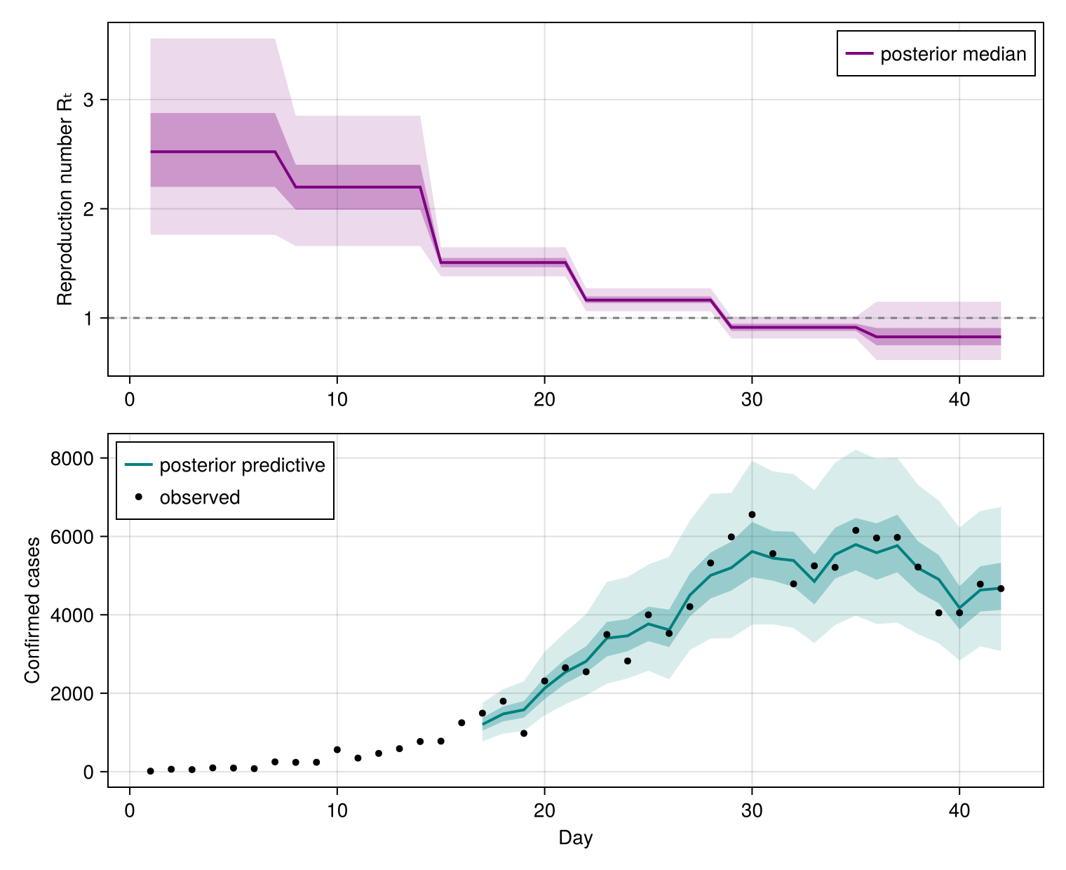

The weekly is piecewise-constant by construction, stepping down through one as the first wave turns over. The posterior-predictive band starts partway into the series — the two delay convolutions leave the earliest reference days without a fully supported expected count — and from there tracks the observed Italian reports, the layered observation model having absorbed the reporting pattern rather than the infection signal.

A time-varying reporting pattern

The day-of-week multiplier above is static: one weekly profile held fixed across the series. Reporting behaviour can itself drift — testing capacity changes, weekend effects strengthen or weaken — and the same composition expresses that. Because the ascertainment modifier takes any latent model, replacing the pooled HierarchicalNormal weekday effect with a BroadcastLatentModel over a process that evolves week to week turns the fixed profile into a time-varying one, at the cost of more latent parameters. The structural change is again local to the observation model; the infection and latent parts are untouched. We keep the static pattern here — it is identifiable from six weeks of data, where a fully time-varying weekday process would not be — and flag the richer variant rather than fit it.

References

2. S. Abbott, J. Hellewell, R. N. Thompson, K. Sherratt, H. P. Gibbs, N. I. Bosse, J. D. Munday, S. Meakin, E. L. Doughty, J. Y. Chun and others. Estimating the time-varying reproduction number of SARS-CoV-2 using national and subnational case counts. Wellcome Open Research 5, 112 (2020).