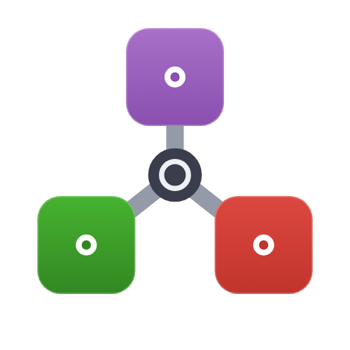
Composable design

ComposableTuringIDModels treats an epidemiological model as a composition of independent parts. A full model has two top-level parts.

• An infection model generates unobserved infections . It owns a latent model internally, an unobserved process such as a log reproduction number or growth rate, which it maps to .

• An observation model maps infections to the observed data .

A latent model describes an unobserved process over time. It is not a mandatory top-level component. The latent is not always the estimand, so it is folded into the infection model that consumes it. You choose an infection model and hand it whatever latent process you want to drive it. Only the Renewal model then carries a generation interval.

Every part is a plain struct that implements a single method of the generic constructor as_turing_model. There is no deep type hierarchy. A part is identified by the method it implements, not by its place in a tree.

One constructor, composed by submodels

as_turing_model(component, args...) returns a DynamicPPL.Model. A component that contains another component builds the inner model and samples it as a submodel.

z ~ as_turing_submodel(inner_model, n)

as_turing_submodel disables automatic variable prefixing by default, so parameter names stay flat. Pass prefix = true to namespace a slot.

Every component speaks the same as_turing_model protocol, so components nest freely. An AR process can carry a HierarchicalNormal error model, a DiffLatentModel can wrap that AR to produce an ARIMA-style process, and that whole latent process can be folded into a DirectInfections model observed with a NegativeBinomialError.

Parameter names, and prefixing where they clash

A component names its own parameters for what they are rather than for which component owns them. An initial value is init, a damping coefficient is damp, a marginal standard deviation is σ. Names stay short because a component knows nothing about what it will be composed with, and a self-describing name would be wrong as soon as the same component appeared twice.

The cost is that two components can want the same name. A Gaussian process draws a marginal standard deviation σ, and so does NormalError. Composed bare, both reach the top level of the same model and land on one variable.

using ComposableTuringIDModels, Distributions
using DynamicPPL: DebugUtils, VarInfo

renewal(rt) = Renewal(;
    generation_time = [0.3, 0.4, 0.3], rt = rt, initialisation = Normal())
bare = as_turing_model(
    IDModel(renewal(HilbertSpaceGP()), NormalError()), fill(10.0, 20), 20)
keys(VarInfo(bare))

4-element Vector{AbstractPPL.VarName}:
 ℓ
 σ
 β
 init_incidence

There are four names for five parameters.

DebugUtils.check_model(bare; error_on_failure = false)

false

sample runs check_model first and refuses to run a model that fails it.

The fix is a prefix applied where the conflict is, rather than a longer name everywhere. PrefixLatentModel wraps a latent process so its variables are namespaced, and PrefixObservationModel does the same for an observation model.

prefixed = as_turing_model(
    IDModel(
        renewal(PrefixLatentModel(; model = HilbertSpaceGP(), prefix = "gp")),
        NormalError()
    ), fill(10.0, 20), 20)
keys(VarInfo(prefixed))

5-element Vector{AbstractPPL.VarName}:
 gp.ℓ
 gp.σ
 gp.β
 init_incidence
 σ

DebugUtils.check_model(prefixed; error_on_failure = false)

true

The Gaussian process's hyperparameters are now gp.ℓ and gp.σ, and the error model keeps its own σ. A chain reads each by its own path, chain[@varname(gp.σ)], and a value is pinned the same way with fix(prefixed, (gp = (σ = 0.2,),)).

Components that compose several children of the same kind prefix them already, so nothing needs adding there. CombineLatentModels names its components Combine.1, Combine.2 and so on, ConcatLatentModels uses Concat.1, Concat.2, DiffLatentModel namespaces the process it differences under diff, and Split prefixes each observation stream by its name.

The latent is folded into the infection model

The latent process is supplied to the infection model rather than to the composer. An infection model takes a latent slot, Z for DirectInfections and rt for ExpGrowthRate and Renewal, and generates that process internally before mapping it to infections. So as_turing_model for an infection model takes only a series length and returns (; I_t, Z_t). Only Renewal needs a generation interval, so it alone takes one. The others take a transformation directly.

Swap-in, swap-out

A modelling assumption changes by replacing a part, not by rewriting the model. Which tool to reach for depends on how many parts you are aiming at. Rebuilding the assembly with one argument different is the plainest case. That is the right thing when the two models share little. When they share almost everything, derive one from the other.

using ComposableTuringIDModels, Distributions
base = IDModel(
    DirectInfections(; Z = RandomWalk(), initialisation = Normal()),
    PoissonError())

IDModel
├─ infection: DirectInfections
│  └─ Z: RandomWalk
│     └─ ϵ_t: HierarchicalNormal
└─ observation: PoissonError

swap replaces every component matching a predicate. Reach for it when the target is "the error model, wherever it is" rather than a known address.

using ComposableTuringIDModels: swap
negbin = swap(x -> x isa PoissonError ? NegativeBinomialError() : x, base)

IDModel
├─ infection: DirectInfections
│  └─ Z: RandomWalk
│     └─ ϵ_t: HierarchicalNormal
└─ observation: NegativeBinomialError

Accessors.@set replaces one component named by its path. The path is the object's own field path, so a component nested several levels down is one line. A printed tree labels each branch with the _model suffix trimmed, so the infection branch is the infection_model field.

using Accessors
autoregressive = @set base.infection_model.Z = AR()

IDModel
├─ infection: DirectInfections
│  └─ Z: AR
│     └─ ϵ_t: HierarchicalNormal
└─ observation: PoissonError

The target does not have to be an observation model, and it does not have to be a whole component. Changing a prior on a nested component is the case a path handles and a predicate cannot, because a distribution carries no identity to match on.

higher_start = @set base.infection_model.Z.init = Normal(log(2.0), 0.1)
higher_start.infection_model.Z.init

Distributions.Normal{Float64}(μ=0.6931471805599453, σ=0.1)

A path also reaches one branch of a Split, and everything wrapped around it comes through untouched, down to a LatentDelay's stored pmf.

split_obs = LatentDelay(
    Split((cases = PoissonError(), deaths = PoissonError())), [0.5, 0.3, 0.2])
deaths_negbin = @set split_obs.model.streams.deaths = NegativeBinomialError()

LatentDelay
└─ model: Split
   ├─ cases: PoissonError
   └─ deaths: NegativeBinomialError

Both tools rest on a seam a component author implements rather than one a user calls. swap walks a chain with ComposableTuringIDModels.wrapped_models and rebuilds it with ComposableTuringIDModels.rewrap. @set goes through ConstructionBase.constructorof, which a component whose public constructor derives a field defines for itself. Inspecting and updating an observation chain covers the walk and both seams.

Composing accumulation steps

The recurrences that drive the time series are expressed as accumulate_scan steps. Within the renewal family these steps compose. A RenewalStep is a force-of-infection core plus an ordered tuple of modifiers that share one incidence window. The first modifier, SusceptibleDepletion, scales the proposed incidence by the available susceptible fraction and depletes the pool, turning the renewal process into one with a fixed population. Renewal is a step-composing helper, so passing the modifier composes it onto the step.

gen_int = [0.2, 0.3, 0.5]

depleting = Renewal(gen_int, SusceptibleDepletion(1000.0); rt = RandomWalk())

Renewal
└─ rt: RandomWalk
   └─ ϵ_t: HierarchicalNormal

A scan step is a deterministic function, so a modifier that needs sampled parameters, an importation rate say, draws them before the scan runs. That is the modifier's optional as_turing_model(mod, n) method, which samples through the same as_turing_submodel seam as everything else and returns the modifier the scan uses. Modifiers that sample nothing return themselves, so the step resolves its whole modifier tuple through one call and nothing in the renewal model tests what a modifier is. ImportedCases is the worked example, and modifiers apply in the order given.

seeded = Renewal(gen_int, SusceptibleDepletion(1000.0),
    ImportedCases(Normal(0.0, 1.0)); rt = RandomWalk())

Renewal
└─ rt: RandomWalk
   └─ ϵ_t: HierarchicalNormal

The generation time is a slot like any other, so a modifier composes onto a continuous generation time the constructor discretises for you. The discretisation keywords stay available alongside the modifiers, which keeps one discretisation path rather than a second one written outside the package.

discretised = Renewal(Gamma(2, 1.5), SusceptibleDepletion(1000.0);
    D_gen = 15.0, rt = RandomWalk())

Renewal
└─ rt: RandomWalk
   └─ ϵ_t: HierarchicalNormal

See Renewal modifiers for what each contributes to a fitted model.

The seeding window

A renewal process needs infections before the modelled window starts. By default initialisation is a level at , one value decaying backwards at the growth rate implied by . Wrapping a process in a SeedingPath estimates that run-up instead, so the data inform its shape rather than fixing it.

seeding = Renewal(; generation_time = gen_int, rt = RandomWalk(),
    initialisation = SeedingPath(RandomWalk(; init = Normal(log(50), 0.5))))
as_turing_model(seeding, 20)().I_seed

3-element Vector{Float64}:
 51.843819436707435
 50.282802529021865
 49.62402258820283

The window is returned as I_seed, whether it was drawn or decayed, and is not part of I_t.

Inference

A composed model is an ordinary Turing model. Pass observed data instead of missing to condition it, then sample. We set the automatic-differentiation backend explicitly with NUTS(; adtype = ...). Mooncake is the recommended default for this package, described under Automatic differentiation backend.

using Turing, Mooncake
using ADTypes: AutoMooncake
y = as_turing_model(base, fill(missing, 30), 30)().generated_y_t
posterior = as_turing_model(base, y, 30)
chain = sample(posterior, NUTS(; adtype = AutoMooncake(; config = nothing)),
    MCMCThreads(), 1_000, 2)

The standard Turing tools all apply unchanged: rand for prior draws, fix to pin parameters, condition to condition on values, and sample for inference.

What data a model needs

The n passed to as_turing_model is the number of observations. That is not always the length of the infection series behind it. Every LatentDelay in an observation chain convolves the expected series with a delay PMF and returns a series shorter by length(pmf) - 1.

The model reads the chain's lead-in, runs the infection process over n + lead_in time points, and hands the observation model exactly n expected values, so every observation is scored. observation_lead_in reads the number off an assembled model, and data_requirements reports what a caller must supply:

delayed = LatentDelay(
    LatentDelay(PoissonError(), fill(1 / 15, 15)), fill(1 / 30, 30))
y = fill(10, 60)

observation_lead_in(delayed)

43

data_requirements(delayed, y, length(y))

DataRequirements: 60 observations per stream
  infection series built at length 103
  y_t: 60 values, after a lead-in of 43 — supplied 60

data_fits is the same question as a yes or no. It asks whether every observation supplied would be scored, so more data than the model can score is false, and supplying that number to as_turing_model is an error.

data_fits(delayed, y, length(y)), data_fits(delayed, vcat(y, y), length(y))

(true, false)

An IDProblem's tspan is the span of the observations for the same reason, and forecast extends the observations by the horizon and derives the rest.

Length-preserving modifiers (Ascertainment, RightTruncate, ReportTriangle, a Split's streams) consume nothing of their own, so the lead-in comes from the delays alone. A Split's streams run in parallel, so their lead-ins do not add up and the series covers the deepest of them. A stream with a shorter lead-in is then handed more expected values than n, which the report says as up to. Supply n for every stream and every one is scored, or supply the extra earlier values for that stream if you have them.

What a stream asks for follows the model that scores it, not the shape of the data. A BinomialError takes (y = successes, N = trials), a ReportTriangle a reference-day × delay matrix counted down its reference days, and an Aggregate a full series of which only the reporting windows are scored. Printing the requirements says which, per stream.

Infection↔observation mappings

An infection model does not have to generate a single curve. Two components widen I_t to an inf_strata x time matrix, one row per stratum.

• Stratify puts a stratum axis on one shared process, combining a shared path with a per-stratum deviation. This is a partially pooled panel, the "same many" case.

• CombineInfections draws several distinct infection processes independently and stacks them. This is the "different many" case, such as a region-level epidemic where each region's curve is genuinely its own process.

On the observation side, Split reads that matrix and projects it onto observation streams through an optional StrataMap obs_strata x inf_strata weight. One mechanism therefore covers every mapping cardinality. map = I is one-to-one, an aggregation row is many-to-one, and a general matrix is many-to-many. Build the infection side with Stratify and pass it straight to the plain IDModel(infection_model, observation_model) constructor. See Partial pooling across groups and Multiple observation streams for worked examples.

Inspecting and updating an observation chain

An observation model is a nesting of modifiers around an error model, each holding what it wraps in a field, so a chain with a few modifiers is several levels deep. Displaying one prints the whole tree.

using ComposableTuringIDModels, Distributions
obs = LatentDelay(
    Ascertainment(
        Split((cases = PoissonError(), deaths = PoissonError())),
        FixedIntercept(log(0.1))
    ),
    [0.5, 0.3, 0.2]
)

LatentDelay
└─ model: Ascertainment
   ├─ model: Split
   │  ├─ cases: PoissonError
   │  └─ deaths: PoissonError
   └─ latent: PrefixLatentModel
      └─ model: FixedIntercept

Reading a component out of that structure without knowing where it sits goes through a walk rather than a field path. ComposableTuringIDModels.wrapped_models reports what a single component wraps. ComposableTuringIDModels.observation_components is the walk built on it, giving every component of a chain outermost first, with a Split's branches followed in stream order. Both are public but not exported, so they are reached through the module name.

Locating a component is a filter over the walk.

using ComposableTuringIDModels: observation_components
delays = filter(x -> x isa LatentDelay, observation_components(obs))
only(delays).delay

3-element Vector{Float64}:
 0.5
 0.3
 0.2

A quantity accumulated over a chain is a sum over the same walk. A quantity that does not accumulate reads the branching structure through wrapped_models instead, because a Split's streams run in parallel off one expected series rather than nesting.

ComposableTuringIDModels.rewrap is the other direction, rebuilding the same wrapper around new wrapped models with everything else it holds carried across. swap is those two together, applied to every component matching a predicate.

using ComposableTuringIDModels: swap
swapped = swap(x -> x isa PoissonError ? NegativeBinomialError() : x, obs)

LatentDelay
└─ model: Ascertainment
   ├─ model: Split
   │  ├─ cases: NegativeBinomialError
   │  └─ deaths: NegativeBinomialError
   └─ latent: PrefixLatentModel
      └─ model: FixedIntercept

Neither is what you call to change one known component. That is Accessors.@set on its path, as in Swap-in, swap-out, and it reaches one stream of a Split the same way.

using Accessors
one_swapped = @set obs.model.model.streams.deaths = NegativeBinomialError()

LatentDelay
└─ model: Ascertainment
   ├─ model: Split
   │  ├─ cases: PoissonError
   │  └─ deaths: NegativeBinomialError
   └─ latent: PrefixLatentModel
      └─ model: FixedIntercept

Several components derive a field from the others on construction. Ascertainment stores its prior already wrapped in a PrefixLatentModel, Aggregate derives its presence mask from its window lengths, and Renewal bakes its accumulation step from the generation interval, the coupling operator and the modifiers. None of them declares a ConstructionBase.constructorof. Two properties make that unnecessary. 2. The derivation is idempotent, so applying it to its own output changes nothing.

3. It runs in the constructor taking the fields in declaration order, which is the one a rebuild calls.

A rebuild from the stored fields then re-derives and lands back where it started. The same constructor gives a field set with Accessors.@set the component the derivation implies. Setting an ascertainment prior re-applies the prefixing, and setting a generation interval, a coupling operator or a modifier re-bakes the step. The package already relies on this for path_prior, which widens a bare Distribution in a path slot. The same reasoning covers every other derived field.

A field that is not stored is better still. HierarchicalNormal adds its mean only when it is non-zero and makes that test where it is used, so no stored flag can disagree with mean.

A modifier defined outside the package inherits both functions as long as it holds what it wraps in its own field. One that holds it somewhere the field walk cannot see, such as inside a container, must define wrapped_models and rewrap for itself. One that derives a field needs only the two properties above. A constructor that cannot accept its own stored fields back is the thing to fix, not to work around.