
Renewal model with negative-binomial reporting
The renewal equation is the workhorse of real-time epidemic estimation: it expresses new infections as a function of past infections weighted by the generation interval, scaled by a time-varying reproduction number
This case study builds that model from two composed parts — a Renewal infection process that carries an autoregressive latent process for NegativeBinomialError observation model — and fits it to the test-confirmed COVID-19 cases from South Korea that Mishra et al. [2] analysed. The latent
The model
Components
The latent process is a second-order autoregressive model on HierarchicalNormal innovation term, matching Mishra et al. [2]. Strong autocorrelation in the reproduction number is encoded by a first damping prior concentrated near one (
using ComposableTuringIDModels, Distributions, Random, Turing, Mooncake
using ADTypes: AutoMooncake
Random.seed!(1234)

latent = AR(
    damp_priors = [truncated(Normal(0.8, 0.05), 0, 1),
        truncated(Normal(0.1, 0.05), 0, 1)],
    init_priors = [Normal(0.0, 0.2), Normal(0.0, 0.2)],
    ϵ_t = HierarchicalNormal(std_prior = HalfNormal(0.1)))
AR
└─ ϵ_t: HierarchicalNormalThe infection process needs a discrete generation interval. IDData takes a continuous distribution and discretises it with double interval censoring [7], using CensoredDistributions.jl. Following Mishra et al. [2] we use a
data = IDData(gen_distribution = Gamma(6.5, 0.62))
data.gen_int
8-element Vector{Float64}:
0.026663134095601098
0.14059778064943768
0.2502660305615845
0.24789569560506872
0.1731751163417783
0.09635404000022221
0.045734375752163825
0.01931382699414364The stored gen_int is a probability vector — the continuous serial interval binned into daily weights that sum to one. Double interval censoring is not the same as evaluating the continuous density at integer days: it accounts for both the primary and secondary events falling anywhere within their days, which shifts and spreads the mass relative to the underlying
sum(data.gen_int), length(data.gen_int)(0.9999999999999999, 8)The Renewal process couples that generation interval to the latent rt slot) and a prior for the initial infections. Renewal is the only infection model that carries an IDData, because it is the only one that uses a generation interval.
renewal = Renewal(data; rt = latent, initialisation_prior = Normal(log(1.0), 0.1))The infection process in isolation
Because the renewal model is a model in its own right, it can be exercised on its own — without an observation model — and we can isolate the contribution of the renewal equation by pinning its reproduction-number process to a known trajectory. With the latent folded in, the way to do that is to build a renewal model whose rt slot is a deterministic FixedIntercept latent, giving a constant as_turing_model call that composes into the full model then runs the infection process standalone, returning its infections I_t and the internal latent draw Z_t.
fixed_logR = log(1.4)
renewal_fixed = Renewal(data;
    rt = FixedIntercept(fixed_logR), initialisation_prior = Normal())
demo = fix(as_turing_model(renewal_fixed, 60), (init_incidence = 0.0,))()
(constant_Rt = round(exp(first(demo.Z_t)), digits = 2),
    grows = demo.I_t[end] > demo.I_t[1])
(constant_Rt = 1.4, grows = true)A constant FixedIntercept latent for a deterministic latent of the desired shape. Nothing here is conditioned on data; the component is inspected in isolation before it is assembled into the full model with its sampled
Reported cases are overdispersed counts of the latent infections. The prior is placed on the cluster factor
obs = NegativeBinomialError(cluster_factor_prior = HalfNormal(0.1))IDModel assembles the two parts — the renewal infection process (which already carries the latent
model = IDModel(renewal, obs)IDModel
├─ infection: Renewal
│ └─ rt: AR
│ └─ ϵ_t: HierarchicalNormal
└─ observation: NegativeBinomialErrorBefore fitting, the composed model is also a prior simulator: passing missing observations makes as_turing_model return generated quantities — the reported cases generated_y_t, the latent infections I_t, and the latent process Z_t — instead of conditioning on data. That is the mechanism used for the prior checks above; here we go straight to real data.
The data
Mishra et al. [2] fit this model to daily test-confirmed COVID-19 cases in South Korea over the first wave of 2020. The series is stored with the docs and read with CSV/DataFrames.
using CSV, DataFrames
datapath = joinpath(pkgdir(ComposableTuringIDModels),
    "docs", "src", "case-studies", "data", "south_korea_data.csv")
south_korea = CSV.read(datapath, DataFrame)
first(south_korea, 5)| Row | Column1 | date | cases_new | deaths_new |
|---|---|---|---|---|
| Int64 | Date | Int64 | Int64 | |
| 1 | 1 | 2019-12-31 | 0 | 0 |
| 2 | 2 | 2020-01-01 | 0 | 0 |
| 3 | 3 | 2020-01-02 | 0 | 0 |
| 4 | 4 | 2020-01-03 | 0 | 0 |
| 5 | 5 | 2020-01-04 | 0 | 0 |
We fit the growth-and-decline window of the first wave, matching the span used by Mishra et al. [2], and take the reported cases over it as the observed series.
tspan = (45, 80)
y_obs = south_korea.cases_new[first(tspan):last(tspan)]
n = length(y_obs)
(n = n, total_cases = sum(y_obs),
    from = south_korea.date[first(tspan)], to = south_korea.date[last(tspan)])
(n = 36, total_cases = 8537, from = Dates.Date("2020-02-13"), to = Dates.Date("2020-03-19"))Fit
Conditioning on the observed counts and sampling with NUTS recovers the posterior. We draw two chains in parallel with MCMCThreads() so the posterior is well resolved and the cross-chain
posterior = as_turing_model(model, y_obs, n)
chain = sample(
    posterior, NUTS(0.9; adtype = AutoMooncake(; config = nothing)),
    MCMCThreads(), 500, 2; progress = false)
┌ Warning: Only a single thread available: MCMC chains are not sampled in parallel
└ @ AbstractMCMC ~/.julia/packages/AbstractMCMC/C1aKp/src/sample.jl:544
┌ Info: Found initial step size
└ ϵ = 0.003125
┌ Warning: There were 41 divergent transitions. Consider reparameterising your model or using a smaller step size. For adaptive samplers such as NUTS and HMCDA, consider increasing `target_accept`.
└ @ Turing.Inference ~/.julia/packages/Turing/4hMHm/src/mcmc/hmc.jl:483
┌ Info: Found initial step size
└ ϵ = 0.0015625
┌ Warning: There were 52 divergent transitions. Consider reparameterising your model or using a smaller step size. For adaptive samplers such as NUTS and HMCDA, consider increasing `target_accept`.
└ @ Turing.Inference ~/.julia/packages/Turing/4hMHm/src/mcmc/hmc.jl:483
┌ Warning: There were 93 divergent transitions. Consider reparameterising your model or using a smaller step size. For adaptive samplers such as NUTS and HMCDA, consider increasing `target_accept`.
└ @ Turing.Inference ~/.julia/packages/Turing/4hMHm/src/mcmc/hmc.jl:483Sampling returns a chain whose parameters keep their flat component names (prefixing is disabled throughout the package). sample returns a FlexiChains chain, which summarystats summarises directly — no conversion step — giving point estimates and their uncertainty alongside the effective sample size and damp_AR[1]), the innovation scale std), and the observation cluster factor cluster_factor) are all identified from the observed South Korean series:
using MCMCChains
summarystats(chain)╭─FlexiSummary (9 statistics) ─────────────────────────────────────────────────╮
│ iter collapsed │
│ chain collapsed │
│ ↓ stat = [mean, std, mcse, ess_bulk, ess_tail, rhat, q5, q50, q95] │
│ │
│ Parameters (41) ── AbstractPPL.VarName │
│ Float64 ar_init[1], ar_init[2], damp_AR[1], damp_AR[2], std, ϵ_t[1], │
│ ϵ_t[2], ϵ_t[3], ϵ_t[4], ϵ_t[5], ϵ_t[6], ϵ_t[7], ϵ_t[8], ϵ_t[9], │
│ ϵ_t[10], ϵ_t[11], ϵ_t[12], ϵ_t[13], ϵ_t[14], ϵ_t[15], ϵ_t[16], │
│ ϵ_t[17], ϵ_t[18], ϵ_t[19], ϵ_t[20], ϵ_t[21], ϵ_t[22], ϵ_t[23], │
│ ϵ_t[24], ϵ_t[25], ϵ_t[26], ϵ_t[27], ϵ_t[28], ϵ_t[29], ϵ_t[30], │
│ ϵ_t[31], ϵ_t[32], ϵ_t[33], ϵ_t[34], init_incidence, │
│ cluster_factor │
│ │
│ Extras (14) │
│ Float64 n_steps, is_accept, acceptance_rate, log_density, │
│ hamiltonian_energy, hamiltonian_energy_error, │
│ max_hamiltonian_energy_error, tree_depth, numerical_error, │
│ step_size, nom_step_size, logprior, loglikelihood, logjoint │
│ │
│ Summary │
│ param mean std mcse ess_bulk ess_tail rhat … │
│ ar_init[1] 0.0230 0.2031 0.0070 817.0863 658.0886 0.9993 … │
│ ar_init[2] -0.0086 0.1993 0.0078 686.9149 405.3150 1.0279 … │
│ damp_AR[1] 0.8137 0.0415 0.0021 397.5913 628.9235 1.0035 … │
│ damp_AR[2] 0.0762 0.0372 0.0020 313.8158 274.2979 1.0050 … │
│ std 0.4178 0.0459 0.0037 157.6087 227.4205 1.0046 … │
│ ϵ_t[1] 0.4825 0.8415 0.0396 460.9003 448.0273 1.0062 … │
│ ϵ_t[2] 0.9504 0.8632 0.0402 469.0098 263.0097 1.0041 … │
│ ϵ_t[3] 1.0895 0.9397 0.0450 448.9361 170.0771 1.0021 … │
│ ϵ_t[4] 1.2966 0.8892 0.0304 858.9271 553.3402 0.9997 … │
│ ϵ_t[5] 2.5425 0.8262 0.0394 438.4231 171.3343 1.0081 … │
│ ϵ_t[6] 1.7069 0.6886 0.0230 903.0302 496.4178 1.0023 … │
│ ϵ_t[7] 0.9116 0.6180 0.0254 593.9195 562.3517 1.0008 … │
│ ϵ_t[8] 0.7140 0.5531 0.0311 312.7008 577.8214 1.0009 … │
│ ϵ_t[9] -0.5565 0.4958 0.0195 651.0417 613.4144 1.0026 … │
│ ϵ_t[10] -2.1831 0.5300 0.0278 361.0790 415.6126 1.0000 … │
│ ϵ_t[11] -1.6148 0.4850 0.0204 581.5653 440.1261 1.0041 … │
│ ϵ_t[12] 0.5523 0.4482 0.0204 478.8469 452.3359 1.0021 … │
│ ϵ_t[13] 1.0814 0.4477 0.0299 305.4216 191.4660 1.0008 … │
│ ϵ_t[14] 0.0370 0.3997 0.0120 1176.1091 490.9129 1.0038 … │
│ ϵ_t[15] 1.2174 0.4389 0.0329 201.5778 424.8299 1.0028 … │
│ ϵ_t[16] -1.0373 0.4567 0.0236 441.0970 241.5813 0.9993 … │
│ ϵ_t[17] -0.4075 0.3733 0.0151 657.9553 413.1194 1.0159 … │
│ ϵ_t[18] -0.7320 0.3903 0.0154 683.7037 291.9448 1.0118 … │
│ ϵ_t[19] -0.6892 0.3666 0.0145 635.8515 297.2981 1.0077 … │
│ ϵ_t[20] -0.5430 0.3785 0.0156 629.0175 393.7403 1.0054 … │
│ ϵ_t[21] 0.1886 0.4024 0.0217 432.4495 352.9036 1.0129 … │
│ ϵ_t[22] -0.0636 0.3713 0.0107 1322.8710 343.7148 1.0057 … │
│ ϵ_t[23] -0.5234 0.3626 0.0131 733.3272 471.1440 1.0033 … │
│ ϵ_t[24] -0.9095 0.3768 0.0155 648.6897 397.1813 1.0141 … │
│ ϵ_t[25] -1.3379 0.4703 0.0229 496.9781 323.3436 1.0109 … │
│ ϵ_t[26] 0.9558 0.4350 0.0347 180.9396 338.0239 1.0069 … │
│ ϵ_t[27] -1.0880 0.4264 0.0214 404.3324 431.6921 1.0014 … │
│ ϵ_t[28] -0.0099 0.4193 0.0198 499.8204 402.6535 1.0055 … │
│ ϵ_t[29] 0.1587 0.4407 0.0170 681.1214 432.3067 1.0018 … │
│ ϵ_t[30] -0.3347 0.4683 0.0144 1036.2776 647.7138 1.0011 … │
│ ϵ_t[31] 0.1779 0.4468 0.0152 852.6876 383.6552 0.9998 … │
│ ϵ_t[32] 0.5270 0.4468 0.0167 702.3233 444.1898 1.0001 … │
│ ϵ_t[33] 0.6487 0.4520 0.0149 955.6840 425.2537 0.9998 … │
│ ϵ_t[34] 1.2502 0.4552 0.0216 466.0043 546.3012 1.0031 … │
│ init_incide… -0.0384 0.1008 0.0029 1158.4461 557.4618 1.0019 … │
│ cluster_fac… 0.1043 0.0653 0.0087 58.0354 168.1490 1.0396 … │
╰──────────────────────────────────────────────────────────────────────────────╯Prior versus posterior
Before reading the trajectories it is worth asking what the data taught us. Sampling the same model with Prior — ignoring the observations — gives a prior draw over the same parameters, and overlaying it on the posterior shows which parameters moved. We load a Makie backend and PairPlots.jl; the FlexiChains PairPlots extension turns a chain (subset to a few keys with chain[[...]]) into a PairPlots.Series, so prior and posterior overlay on one corner plot.
using CairoMakie, PairPlots

prior_chain = sample(posterior, Prior(), 1000; progress = false)
pp_keys = [@varname(damp_AR), @varname(std),
    @varname(cluster_factor), @varname(init_incidence)]
pairplot(
    PairPlots.Series(chain[pp_keys]; label = "posterior"),
    PairPlots.Series(prior_chain[pp_keys]; label = "prior"))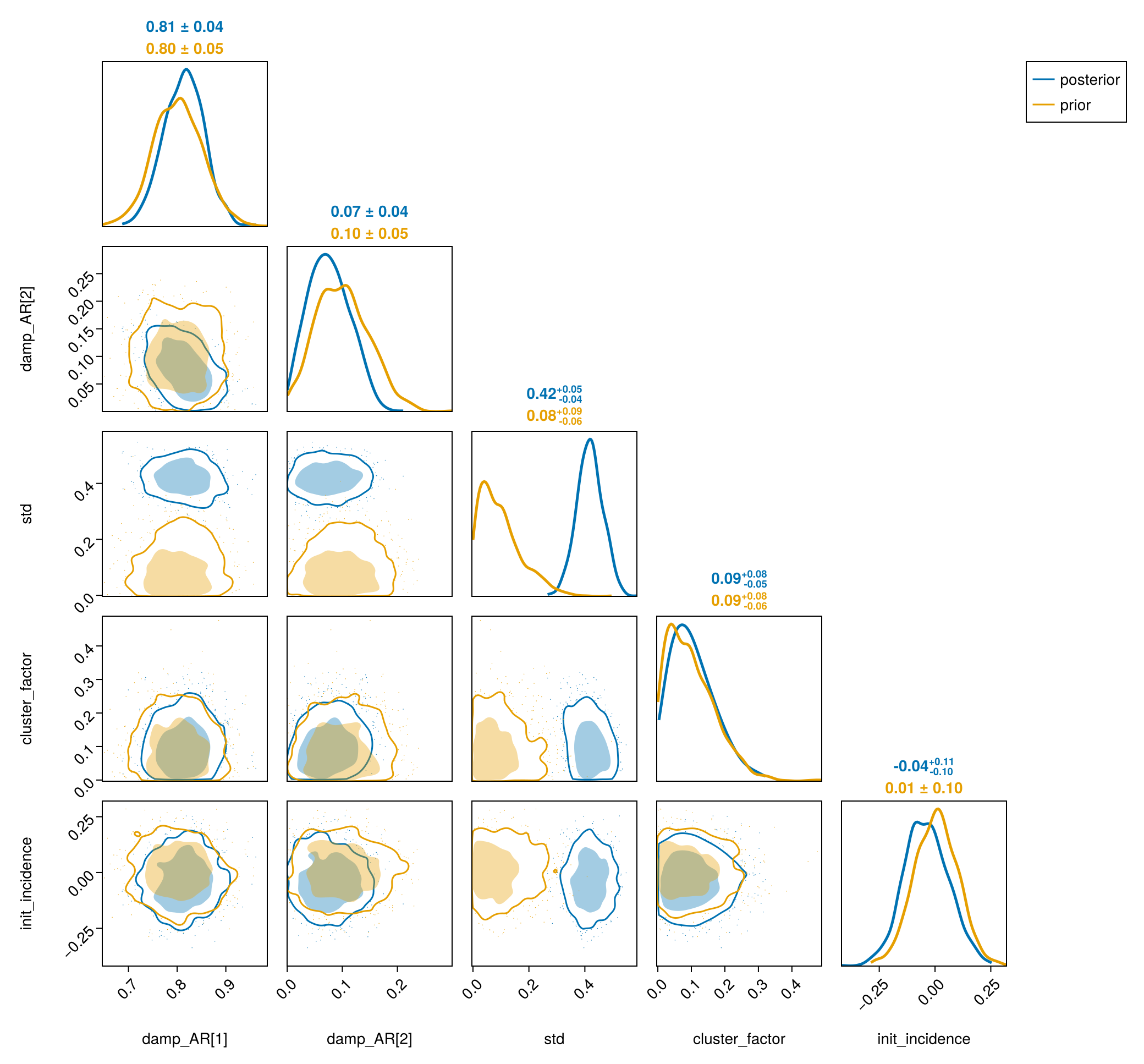
The innovation scale std) is sharply updated away from its prior — the data are informative about how much damp_AR), the cluster factor and the initial infections stay closer to their priors on this short window.
Posterior trajectories
The reproduction number generated_observables re-runs the fitted model over the chain to recover the latent predict on the same model with the observations set to missing.
A couple of small helpers reduce the per-draw trajectories to credible bands and draw a median line with 50% and 95% ribbons.
Stack the per-draw
gens = vec(generated_observables(posterior, y_obs, chain).generated)
Rt = credible_bands(reduce(hcat, (exp.(g.Z_t) for g in gens)))

pred = predict(as_turing_model(model, fill(missing, n), n), chain)
yt = predictive_bands(pred, n)

fig = Figure(; size = (760, 620))
ax1 = Axis(fig[1, 1]; ylabel = "Reproduction number Rₜ")
ci_ribbon!(ax1, 1:size(Rt, 1), Rt; color = :purple, label = "posterior median")
hlines!(ax1, [1.0]; color = :grey, linestyle = :dash)
axislegend(ax1; position = :rt)
ax2 = Axis(fig[2, 1]; xlabel = "Day", ylabel = "Reported cases")
ci_ribbon!(ax2, 1:size(yt, 1), yt; color = :teal,
    label = "posterior predictive")
scatter!(ax2, 1:n, y_obs; color = :black, markersize = 7, label = "observed")
axislegend(ax2; position = :lt)
fig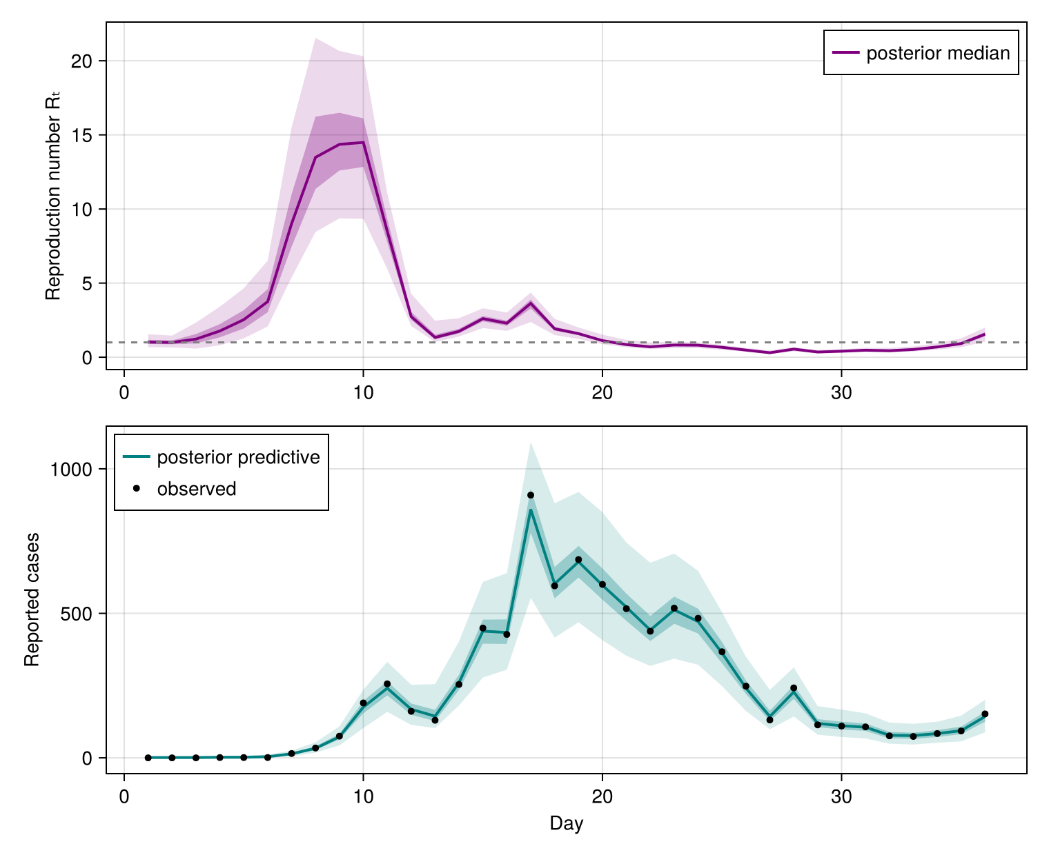
The posterior-predictive band tracks the observed South Korean series closely, and the
Swap a component
Because the parts share one interface, an alternative observation assumption is a one-line change. Swapping the negative-binomial reporting for a PoissonError leaves the renewal infection process — and its latent
poisson_model = IDModel(renewal, PoissonError())
length(rand(as_turing_model(poisson_model, fill(missing, n), n)))41References
A. Cori, N. M. Ferguson, C. Fraser and S. Cauchemez. A new framework and software to estimate time-varying reproduction numbers during epidemics. American Journal of Epidemiology 178, 1505–1512 (2013).
S. Mishra, T. Berah, T. A. Mellan, H. J. Unwin, M. A. Vollmer, K. V. Parag, A. Gandy, S. Flaxman and S. Bhatt. On the derivation of the renewal equation from an age-dependent branching process: an epidemic modelling perspective, arXiv preprint arXiv:2006.16487 (2020).
K. Charniga, S. W. Park, A. R. Akhmetzhanov, A. Cori, J. Dushoff, S. Funk and others. Best practices for estimating and reporting epidemiological delay distributions of infectious diseases. PLoS Computational Biology 20, e1012520 (2024).