
Real-time nowcasting: correcting right-truncation
In real time, the most recent days of a surveillance series are incomplete: a case with reference day
This case study takes a real, fully-reported case series — the daily confirmed COVID-19 cases from Italy's first wave used in the delays example — treats it as the eventual totals, and truncates its recent tail to mimic the real-time snapshot an analyst would have seen mid-outbreak. It then contrasts two fits: a naive one that treats the truncated counts as complete, and one that wraps the observation model in RightTruncate to scale each reference day's expected count by the fraction of its eventual total reported so far. The correction is the EpiNow2-style CDF-scaling nowcast [3], expressed here as a one-line observation modifier.
The idea
The infection pipeline produces RightTruncate conditions the observation error on that down-weighted mean, so the model's
A naive fit drops the
The full-data model
We build the same composed renewal model as the renewal case study: an autoregressive Renewal infection process, observed with a NegativeBinomialError.
using ComposableTuringIDModels, Distributions, Random, Turing
using CSV, DataFrames
Random.seed!(20240625)

latent = AR(
    damp_priors = [truncated(Normal(0.8, 0.05), 0, 1)],
    init_priors = [Normal(0.0, 0.25)],
    ϵ_t = HierarchicalNormal(std_prior = HalfNormal(0.1)))
data = IDData(gen_distribution = Gamma(1.4, 1 / 0.38))
renewal = Renewal(data; rt = latent, initialisation_prior = Normal(log(1.0), 1.0))
error = NegativeBinomialError(cluster_factor_prior = HalfNormal(0.1))
Take a real series and truncate it
We use the fully-reported Italy confirmed-case series as the eventual totals, then impose a reporting delay and truncate at ReportingCDF builds the completeness curve
datapath = joinpath(pkgdir(ComposableTuringIDModels),
    "docs", "src", "case-studies", "data", "italy_data.csv")
italy = CSV.read(datapath, DataFrame)
n = 50
eventual = italy.confirm[1:n]                # the eventual (complete) totals

reporting_delay = LogNormal(1.6, 0.5)        # mean ≈ 5.6 days
cdf_curve = ReportingCDF(reporting_delay)
Now form the right-truncated snapshot: thin each reference day's eventual total to the fraction reported by
completeness = as_turing_model(cdf_curve, n)()    # F by age, F[1] = age 0
scale = reverse(completeness)                     # by reference day t = 1..n
observed_so_far = @. rand(Binomial(eventual, scale))
(complete_tail = eventual[(end - 4):end], truncated_tail = observed_so_far[(end - 4):end])
(complete_tail = [3599, 3039, 3836, 4204, 3951], truncated_tail = [1497, 752, 355, 64, 0])The last few days are visibly thinned: the most recent day shows only a fraction of its eventual count.
Fit 1 — naive (no truncation correction)
Condition the plain renewal model on the truncated counts as though they were complete.
naive_model = IDModel(renewal, error)
naive_post = as_turing_model(naive_model, observed_so_far, n)
naive_chain = sample(
    naive_post, NUTS(0.9), MCMCThreads(), 500, 2; progress = false)
┌ Warning: Only a single thread available: MCMC chains are not sampled in parallel
└ @ AbstractMCMC ~/.julia/packages/AbstractMCMC/C1aKp/src/sample.jl:544
┌ Info: Found initial step size
└ ϵ = 0.00625
┌ Warning: There were 7 divergent transitions. Consider reparameterising your model or using a smaller step size. For adaptive samplers such as NUTS and HMCDA, consider increasing `target_accept`.
└ @ Turing.Inference ~/.julia/packages/Turing/4hMHm/src/mcmc/hmc.jl:483
┌ Info: Found initial step size
└ ϵ = 0.003125
┌ Warning: There were 39 divergent transitions. Consider reparameterising your model or using a smaller step size. For adaptive samplers such as NUTS and HMCDA, consider increasing `target_accept`.
└ @ Turing.Inference ~/.julia/packages/Turing/4hMHm/src/mcmc/hmc.jl:483
┌ Warning: There were 46 divergent transitions. Consider reparameterising your model or using a smaller step size. For adaptive samplers such as NUTS and HMCDA, consider increasing `target_accept`.
└ @ Turing.Inference ~/.julia/packages/Turing/4hMHm/src/mcmc/hmc.jl:483Fit 2 — corrected with RightTruncate
Wrap the same error model in RightTruncate with the same reporting delay. Nothing else changes — the infection process and its latent
corrected_obs = RightTruncate(error, reporting_delay)
corrected_model = IDModel(renewal, corrected_obs)
corrected_post = as_turing_model(corrected_model, observed_so_far, n)
corrected_chain = sample(
    corrected_post, NUTS(0.9), MCMCThreads(), 500, 2; progress = false)
┌ Warning: Only a single thread available: MCMC chains are not sampled in parallel
└ @ AbstractMCMC ~/.julia/packages/AbstractMCMC/C1aKp/src/sample.jl:544
┌ Info: Found initial step size
└ ϵ = 0.0015625
┌ Warning: There were 4 divergent transitions. Consider reparameterising your model or using a smaller step size. For adaptive samplers such as NUTS and HMCDA, consider increasing `target_accept`.
└ @ Turing.Inference ~/.julia/packages/Turing/4hMHm/src/mcmc/hmc.jl:483
┌ Info: Found initial step size
└ ϵ = 0.0125
┌ Warning: There were 1 divergent transitions. Consider reparameterising your model or using a smaller step size. For adaptive samplers such as NUTS and HMCDA, consider increasing `target_accept`.
└ @ Turing.Inference ~/.julia/packages/Turing/4hMHm/src/mcmc/hmc.jl:483
┌ Warning: There were 5 divergent transitions. Consider reparameterising your model or using a smaller step size. For adaptive samplers such as NUTS and HMCDA, consider increasing `target_accept`.
└ @ Turing.Inference ~/.julia/packages/Turing/4hMHm/src/mcmc/hmc.jl:483The right-truncation bias and its correction
The reproduction number returned (re-exported by Turing) recovers the latent RightTruncate fit removes that bias.
using Statistics

function recent_Rt(posterior, chain; window = 7)
    # Per-draw R_t = exp(Z_t); average over draws, then over the recent window.
    gens = vec(returned(posterior, chain))
    Rt_mean = mean(exp.(g.Z_t) for g in gens)
    mean(Rt_mean[(end - window + 1):end])
end

complete_post = as_turing_model(naive_model, eventual, n)
complete_chain = sample(
    complete_post, NUTS(0.9), MCMCThreads(), 500, 2; progress = false)

R_complete_recent = recent_Rt(complete_post, complete_chain)
R_naive_recent = recent_Rt(naive_post, naive_chain)
R_corrected_recent = recent_Rt(corrected_post, corrected_chain)

(complete = round(R_complete_recent, digits = 2),
    naive = round(R_naive_recent, digits = 2),
    corrected = round(R_corrected_recent, digits = 2))
(complete = 0.91, naive = 0.31, corrected = 0.95)The naive recent-RightTruncate fit, which knows the recent days are incomplete, pulls the recent
Prior versus posterior
Sampling the corrected model with Prior gives a prior draw over the shared renewal parameters. Overlaying it on the posterior with PairPlots.jl confirms the truncation correction still identifies them from the thinned tail.
using CairoMakie, PairPlots

prior_chain = sample(corrected_post, Prior(), 1000; progress = false)
pp_keys = [@varname(damp_AR), @varname(std),
    @varname(cluster_factor), @varname(init_incidence)]
pairplot(
    PairPlots.Series(corrected_chain[pp_keys]; label = "posterior"),
    PairPlots.Series(prior_chain[pp_keys]; label = "prior"))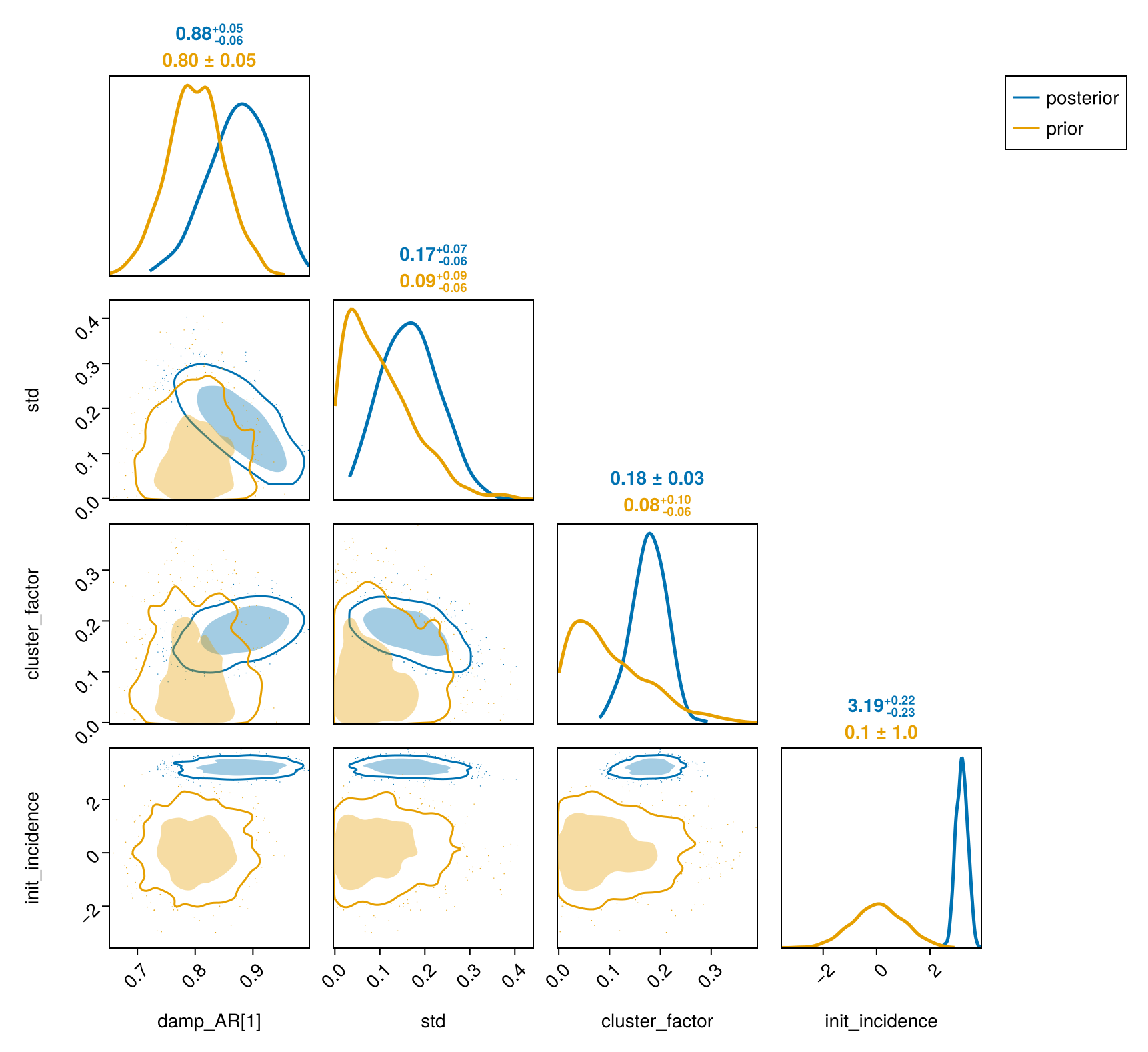
The correction in a figure
generated_observables. Plotting the posterior median and 95% band for all three fits over time — the complete-data reference, the naive truncated fit, and the RightTruncate-corrected fit — shows the right-truncation artefact and its removal in the recent window (shaded).
Rt_complete = rt_bands(complete_post, eventual, complete_chain)
Rt_naive = rt_bands(naive_post, observed_so_far, naive_chain)
Rt_corrected = rt_bands(corrected_post, observed_so_far, corrected_chain)

ts = 1:n
fig = Figure(; size = (760, 420))
ax = Axis(fig[1, 1]; xlabel = "Reference day",
    ylabel = "Reproduction number Rₜ")
vspan!(ax, n - 6, n; color = (:grey, 0.15))
rt_line!(ax, ts, Rt_complete; color = :black, label = "complete (reference)")
rt_line!(ax, ts, Rt_naive; color = :crimson, label = "naive (truncated)")
rt_line!(ax, ts, Rt_corrected; color = :seagreen, label = "corrected")
hlines!(ax, [1.0]; color = :grey, linestyle = :dash)
axislegend(ax; position = :lb)
fig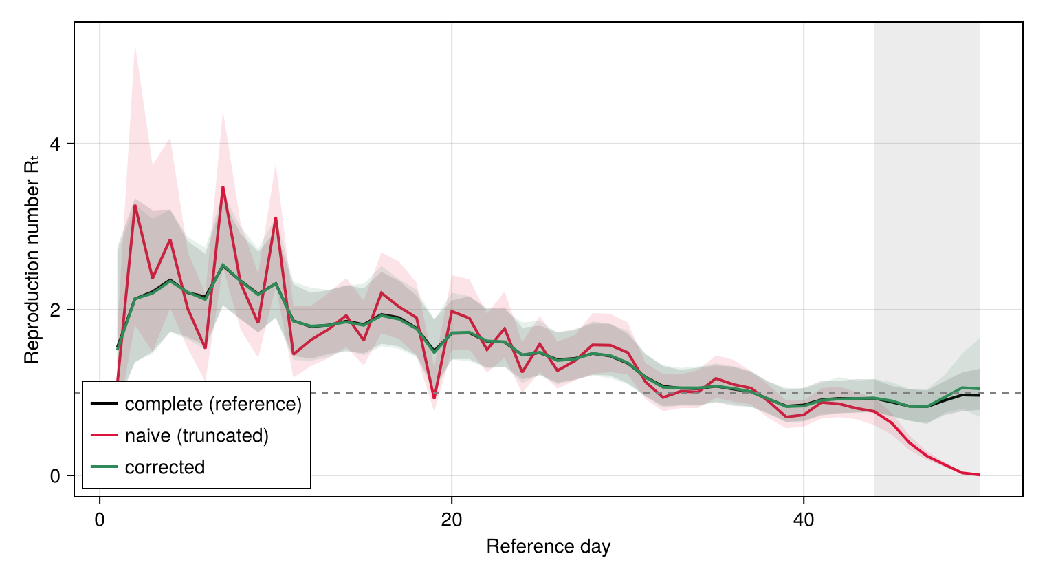
In the shaded recent window the naive fit (red) dips below the complete-data reference (black) — the artefactual late down-turn — while the RightTruncate correction (green) pulls the recent
Reading the shared parameters
Wrapping the error model in RightTruncate does not touch the renewal process, so the corrected fit recovers the same shared parameters: the autoregressive damping damp_AR[1]), the innovation scale std), the observation overdispersion (cluster_factor), and the initial infections (init_incidence). They keep their flat names (prefixing is disabled throughout the package).
sample returns a FlexiChains chain, which summarystats summarises directly — no conversion step — giving point estimates and their uncertainty alongside the effective sample size and
using MCMCChains
summarystats(corrected_chain)╭─FlexiSummary (9 statistics) ─────────────────────────────────────────────────╮
│ iter collapsed │
│ chain collapsed │
│ ↓ stat = [mean, std, mcse, ess_bulk, ess_tail, rhat, q5, q50, q95] │
│ │
│ Parameters (54) ── AbstractPPL.VarName │
│ Float64 ar_init[1], damp_AR[1], std, ϵ_t[1], ϵ_t[2], ϵ_t[3], ϵ_t[4], │
│ ϵ_t[5], ϵ_t[6], ϵ_t[7], ϵ_t[8], ϵ_t[9], ϵ_t[10], ϵ_t[11], ϵ_t[12], │
│ ϵ_t[13], ϵ_t[14], ϵ_t[15], ϵ_t[16], ϵ_t[17], ϵ_t[18], ϵ_t[19], │
│ ϵ_t[20], ϵ_t[21], ϵ_t[22], ϵ_t[23], ϵ_t[24], ϵ_t[25], ϵ_t[26], │
│ ϵ_t[27], ϵ_t[28], ϵ_t[29], ϵ_t[30], ϵ_t[31], ϵ_t[32], ϵ_t[33], │
│ ϵ_t[34], ϵ_t[35], ϵ_t[36], ϵ_t[37], ϵ_t[38], ϵ_t[39], ϵ_t[40], │
│ ϵ_t[41], ϵ_t[42], ϵ_t[43], ϵ_t[44], ϵ_t[45], ϵ_t[46], ϵ_t[47], │
│ ϵ_t[48], ϵ_t[49], init_incidence, cluster_factor │
│ │
│ Extras (14) │
│ Float64 n_steps, is_accept, acceptance_rate, log_density, │
│ hamiltonian_energy, hamiltonian_energy_error, │
│ max_hamiltonian_energy_error, tree_depth, numerical_error, │
│ step_size, nom_step_size, logprior, loglikelihood, logjoint │
│ │
│ Summary │
│ param mean std mcse ess_bulk ess_tail rhat … │
│ ar_init[1] 0.4113 0.3118 0.0251 156.6024 381.3858 1.0032 … │
│ damp_AR[1] 0.8758 0.0518 0.0045 126.9111 221.1110 1.0019 … │
│ std 0.1685 0.0632 0.0067 90.6875 251.5116 1.0051 … │
│ ϵ_t[1] 2.1302 0.9874 0.0658 228.8162 565.2345 0.9995 … │
│ ϵ_t[2] 0.7956 0.8889 0.0343 662.1075 650.1480 1.0013 … │
│ ϵ_t[3] 0.9621 0.8570 0.0259 1136.5229 748.5705 1.0022 … │
│ ϵ_t[4] 0.3003 0.8411 0.0322 699.3578 736.6649 0.9991 … │
│ ϵ_t[5] 0.3391 0.8547 0.0272 982.4369 803.0370 1.0015 … │
│ ϵ_t[6] 1.6274 0.9546 0.0518 350.1411 708.7181 0.9998 … │
│ ϵ_t[7] 0.2194 0.8739 0.0275 974.3717 675.0057 0.9996 … │
│ ϵ_t[8] 0.1734 0.8293 0.0216 1468.8536 762.4451 0.9991 … │
│ ϵ_t[9] 0.9041 0.8654 0.0536 259.4061 601.7201 1.0000 … │
│ ϵ_t[10] -0.7213 0.8526 0.0378 504.3991 531.6581 0.9992 … │
│ ϵ_t[11] 0.2367 0.8275 0.0245 1141.7382 629.2100 0.9998 … │
│ ϵ_t[12] 0.4375 0.8539 0.0283 1008.0792 560.3846 0.9995 … │
│ ϵ_t[13] 0.5345 0.8433 0.0334 643.7635 516.8436 0.9994 … │
│ ϵ_t[14] 0.3542 0.7972 0.0234 1167.8888 621.5683 1.0005 … │
│ ϵ_t[15] 0.8203 0.8141 0.0265 956.2461 843.5450 0.9992 … │
│ ϵ_t[16] 0.3348 0.8427 0.0211 1585.1577 782.7961 1.0066 … │
│ ϵ_t[17] 0.0892 0.7703 0.0234 1086.1232 697.6540 1.0005 … │
│ ϵ_t[18] -0.6908 0.8790 0.0499 318.0032 550.3467 1.0058 … │
│ ϵ_t[19] 1.1875 0.8994 0.0567 245.1267 526.5821 1.0046 … │
│ ϵ_t[20] 0.3739 0.8143 0.0224 1320.9579 743.5999 1.0011 … │
│ ϵ_t[21] 0.0399 0.7787 0.0200 1616.0626 813.1790 1.0127 … │
│ ϵ_t[22] 0.2959 0.7409 0.0272 723.4930 618.4396 1.0007 … │
│ ϵ_t[23] -0.2710 0.7678 0.0247 913.2754 708.5966 1.0031 … │
│ ϵ_t[24] 0.3609 0.8172 0.0284 859.4860 856.5315 0.9998 … │
│ ϵ_t[25] -0.1103 0.7689 0.0251 933.4076 704.8933 1.0079 … │
│ ϵ_t[26] 0.2971 0.7627 0.0252 910.2992 722.0669 1.0073 … │
│ ϵ_t[27] 0.4642 0.7882 0.0281 825.8477 516.1221 1.0002 … │
│ ϵ_t[28] 0.1546 0.7687 0.0250 983.2745 723.5993 1.0016 … │
│ ϵ_t[29] -0.1483 0.7901 0.0241 1065.8966 689.3369 1.0003 … │
│ ϵ_t[30] -0.6003 0.8065 0.0233 1168.1994 743.1565 0.9994 … │
│ ϵ_t[31] -0.5564 0.7665 0.0215 1286.9944 631.2106 1.0044 … │
│ ϵ_t[32] -0.0821 0.7557 0.0267 819.2379 659.1198 0.9990 … │
│ ϵ_t[33] -0.0179 0.8083 0.0262 957.2035 636.5960 1.0010 … │
│ ϵ_t[34] 0.1392 0.7722 0.0271 805.0177 542.0546 1.0051 … │
│ ϵ_t[35] -0.1358 0.7665 0.0287 766.8047 405.3091 1.0023 … │
│ ϵ_t[36] -0.2343 0.7583 0.0238 1032.0819 762.8194 1.0038 … │
│ ϵ_t[37] -0.5802 0.7991 0.0215 1419.0623 602.3870 1.0019 … │
│ ϵ_t[38] -0.6556 0.7694 0.0231 1158.2606 562.5643 1.0095 … │
│ ϵ_t[39] -0.1051 0.7875 0.0225 1247.0222 653.6702 1.0096 … │
│ ϵ_t[40] 0.2991 0.8346 0.0263 1010.4971 837.2983 1.0025 … │
│ ϵ_t[41] 0.0258 0.7862 0.0241 1098.2763 557.3610 1.0007 … │
│ ϵ_t[42] -0.0201 0.7439 0.0220 1130.2675 737.2112 0.9995 … │
│ ϵ_t[43] -0.0182 0.7355 0.0238 960.4390 477.9180 0.9995 … │
│ ϵ_t[44] -0.2582 0.7871 0.0238 1088.5207 642.2759 1.0004 … │
│ ϵ_t[45] -0.5404 0.7838 0.0237 1094.6987 474.1798 1.0040 … │
│ ϵ_t[46] -0.1355 0.8281 0.0287 825.2804 653.2932 1.0022 … │
│ ϵ_t[47] 0.6302 0.7626 0.0217 1225.6248 708.7481 1.0028 … │
│ ϵ_t[48] 0.6142 0.8388 0.0276 941.2357 674.3743 1.0009 … │
│ ϵ_t[49] 0.0063 0.9631 0.0303 1022.6868 649.4251 1.0020 … │
│ init_incide… 3.1893 0.2192 0.0074 890.8789 822.4032 0.9992 … │
│ cluster_fac… 0.1779 0.0339 0.0035 97.1783 117.6702 1.0033 … │
╰──────────────────────────────────────────────────────────────────────────────╯From the marginal to the joint
RightTruncate corrects right-truncation by conditioning on each reference day's observed-so-far total — the marginal of the full reference-day × reporting-delay structure. When the delay structure itself is of interest (e.g. reporting that drifts over the outbreak), the ReportTriangle observation model keeps the full 2D reporting triangle and scores it cell by cell; its observed row-sums reconcile with this CDF-scaling to machine precision. The marginal correction here is the cheaper, released-code first step.
References
- S. Abbott, J. Hellewell, R. N. Thompson, K. Sherratt, H. P. Gibbs, N. I. Bosse, J. D. Munday, S. Meakin, E. L. Doughty, J. Y. Chun and others. Estimating the time-varying reproduction number of SARS-CoV-2 using national and subnational case counts. Wellcome Open Research 5, 112 (2020).