Time-varying damping in an AR process

Every parameter slot of a component takes a raw prior. Which kind of prior you put in the slot decides whether the parameter is constant or time-varying, through one general mechanism that any component can use:

• a bare Distribution gives a constant parameter — one scalar draw, shared across the series (efficient, no length-n allocation); and

• a process (a latent model such as a RandomWalk) gives a time-varying parameter — a whole path, one value per step.

The component reads the parameter the same way at every step (ComposableTuringIDModels._at(ρ, t)), so a single recursion serves both cases. Here we use the damping coefficient of an autoregressive process as the worked example, but the same widening applies to any scalar parameter.

Constant versus time-varying damping

AR with a Distribution damping prior is an ordinary constant-coefficient autoregression — the coefficient is one number for the whole series:

using ComposableTuringIDModels, Distributions, Turing, Random, Statistics
using Turing: to_submodel
Random.seed!(80)

constant = AR(; damp = Normal(0.4, 0.1))
(order = constant.p, coefficient_is_constant = true)

(order = 1, coefficient_is_constant = true)

Swapping the Distribution for a process turns the same slot into a genuinely time-varying coefficient path :

where the unconstrained path is drawn from the process (a RandomWalk here) and tanh maps it into the stationary band  . This is a one-line change to the damp argument — the AR recursion is untouched — and the named constructor TimeVaryingAR is exactly this:

tv = AR(; damp = RandomWalk())          # === TimeVaryingAR()
(order = tv.p, transform = tv.transform)

(order = 1, transform = tanh)

Built with as_turing_model(m, n) it returns the numeric length-n path (like every other latent model), and tracks the coefficient path as a generated quantity ρ (recovered from the chain, below):

length(as_turing_model(tv, 8)())

8

Because it returns a plain path it drops straight into any latent slot — here as the process of a Renewal inside a composed IDModel, with no glue code:

gen_int = [0.2, 0.3, 0.5]
nested = IDModel(
    Renewal(; generation_time = gen_int, rt = AR(; damp = RandomWalk()),
        initialisation = Normal()),
    PoissonError())
length(as_turing_model(nested, missing, 12)().generated_y_t)

12

We simulate one series whose true damping ramps from strong positive persistence through zero to mild anti-persistence, then recover it. A single series informs each through one transition, so recovery leans on the smoothness of the RandomWalk damping prior (a panel of series sharing one draw would sharpen it further):

n = 50
tgrid = range(0, 1; length = n - 1)
ρ_true = 0.85 .- 1.15 .* tgrid          # 0.85 → −0.30, crossing zero
z = zeros(n)
z[1] = randn()
for t in 2:n
    z[t] = ρ_true[t - 1] * z[t - 1] + 0.3 * randn()
end
(n = n, ρ_start = round(ρ_true[1], digits = 2),
    ρ_end = round(ρ_true[end], digits = 2))

(n = 50, ρ_start = 0.85, ρ_end = -0.3)

The model wraps the time-varying AR in a thin observation of the path and fits under NUTS. The coefficient path is tracked as the generated quantity ρ, so it is recovered straight from the chain:

@model function observe_path(y, n)
    latent ~ as_turing_submodel(AR(; damp = RandomWalk()), n)
    for t in 1:n
        y[t] ~ Normal(latent[t], 0.01)
    end
end

model = observe_path(z, n)
fit = sample(model, NUTS(0.85; adtype = Turing.AutoForwardDiff()), 300;
    progress = false)
# ρ is tracked as a generated quantity: `fit[:ρ]` is a per-draw coefficient path
ρ_draws = reduce(hcat, vec(fit[:ρ]))     # (n-1) × draws
ρ_mean = vec(mean(ρ_draws; dims = 2))
(correlation_with_truth = round(cor(ρ_mean, ρ_true), digits = 2),)

(correlation_with_truth = 0.68,)

The posterior mean damping path tracks the true ramp, including the sign change. Plotting it against the truth with an 80% credible band makes the recovery visible:

using CairoMakie
qs = [quantile(ρ_draws[t, :], [0.1, 0.5, 0.9]) for t in 1:(n - 1)]
lo = getindex.(qs, 1)
md = getindex.(qs, 2)
hi = getindex.(qs, 3)

fig = Figure(; size = (760, 420))
ax = Axis(fig[1, 1]; xlabel = "Time step", ylabel = "Damping ρₜ")
band!(ax, 1:(n - 1), lo, hi; color = (:seagreen, 0.25))
lines!(ax, 1:(n - 1), md; color = :seagreen, linewidth = 2,
    label = "posterior mean")
lines!(ax, 1:(n - 1), ρ_true; color = :black, linestyle = :dash, linewidth = 2,
    label = "true ρₜ")
hlines!(ax, [0.0]; color = :grey, linestyle = :dot)
axislegend(ax; position = :lb)
fig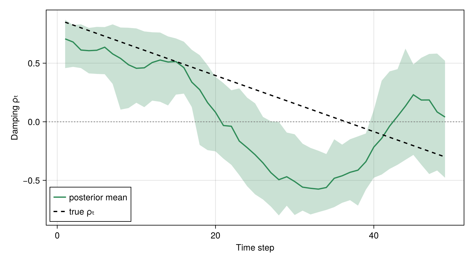

The band covers the true trajectory across the series, so the time-varying damping is recovered from data — with the coefficient's evolution supplied as an ordinary prior process rather than coded by hand. The same mechanism widens any scalar parameter to a time-varying one: put a process in its slot instead of a Distribution. Only the order-1 case is built so far; time-varying coefficients for higher-order AR(p) are tracked in #113.