Renewal modifiers: susceptible depletion and importation

A Renewal process can be extended by modifiers that change how the next incidence is formed. This page takes one delayed renewal process and adds two of them — SusceptibleDepletion, which bounds the epidemic by a finite population, and ImportedCases, which seeds infections from outside it — so the contribution of each is visible against the same baseline.

Everything else is held fixed: the same generation interval, the same reproduction number, the same reporting delay, and the same initial incidence. Only the modifier list changes.

using ComposableTuringIDModels, Distributions, Random, Turing, Mooncake
using CairoMakie
using ADTypes: AutoMooncake
using DynamicPPL: fix
using Statistics: quantile

Random.seed!(20260727)

A delayed renewal process

The infection process is a renewal equation with a discretised generation interval and a constant  . Fixing with a FixedIntercept keeps the comparison clean: any difference between the runs below is the modifiers' doing, not a different draw of the reproduction number.

gen_int = [0.2, 0.3, 0.3, 0.2]
n = 60
pop_size = 2_000.0

function renewal(modifiers...)
    Renewal(gen_int, modifiers...;
        rt = FixedIntercept(log(1.3)), initialisation = Normal())
end

Reported cases are the infections convolved with a reporting delay and observed with negative-binomial noise — a LatentDelay wrapped around a NegativeBinomialError.

delay = [0.1, 0.4, 0.3, 0.2]
obs = LatentDelay(
    NegativeBinomialError(cluster_factor = HalfNormal(0.1)), delay)

LatentDelay
└─ model: NegativeBinomialError

Three models

The three models differ only in the modifiers composed onto the renewal step. Modifiers apply in the order given, so importation here is added after depletion: imported infections are not scaled by the susceptible fraction and do not themselves deplete the pool.

models = (
    plain = IDModel(renewal(), obs),
    depleting = IDModel(renewal(SusceptibleDepletion(pop_size)), obs),
    seeded = IDModel(
        renewal(SusceptibleDepletion(pop_size),
            ImportedCases(FixedIntercept(log(2.0)))),
        obs))

Simulating from each model with missing observations and the same fixed initial incidence returns its infections and reported cases.

simulate(model) = fix(as_turing_model(model, missing, n),
    (init_incidence = log(1.0),))()

sims = map(simulate, models)

What each modifier does

Both panels use a log scale; the reported counts in the lower panel are floored at one so that zero-report days stay visible. The reporting delay leaves the first length(delay) - 1 days without a reported count, so the lower panel starts on day length(delay).

obs_days = length(delay):n

fig = Figure(; size = (760, 560))
ax1 = Axis(fig[1, 1]; ylabel = "Infections Iₜ", yscale = log10)
ax2 = Axis(fig[2, 1]; xlabel = "Day", ylabel = "Reported cases", yscale = log10)
colours = (plain = :grey30, depleting = :purple, seeded = :teal)
labels = (plain = "renewal", depleting = "+ susceptible depletion",
    seeded = "+ importation")
for k in keys(sims)
    lines!(ax1, 1:n, sims[k].I_t; color = colours[k], linewidth = 2,
        label = labels[k])
    scatter!(ax2, obs_days, max.(sims[k].generated_y_t[obs_days], 1);
        color = colours[k], markersize = 7)
end
axislegend(ax1; position = :lt)
fig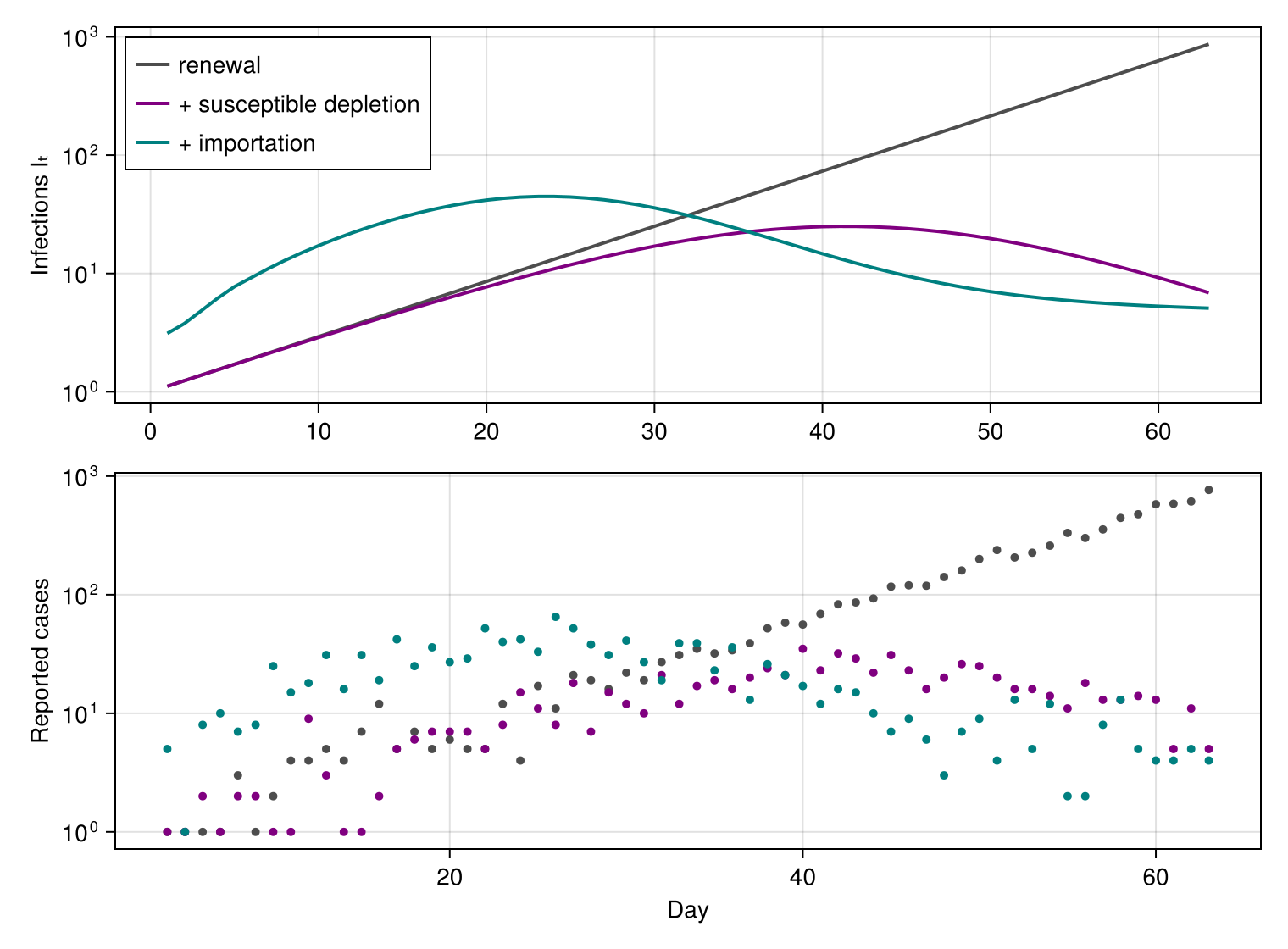

The plain renewal grows exponentially without bound. Susceptible depletion turns that growth over: as susceptibles are used up the effective reproduction number falls below one, so incidence peaks and declines. Importation keeps seeding the epidemic instead of leaving it to grow from the initial incidence alone, which front-loads it, so it peaks earlier and higher and spends the susceptible pool sooner.

function summarise(sim)
    (; peak_day = argmax(sim.I_t),
        peak = round(maximum(sim.I_t); digits = 1),
        final = round(last(sim.I_t); digits = 1))
end
map(summarise, (depleting = sims.depleting, seeded = sims.seeded))

(depleting = (peak_day = 41, peak = 25.0, final = 9.2), seeded = (peak_day = 24, peak = 44.7, final = 5.3))

Late incidence in the seeded run is therefore the lower of the two, its epidemic already past.

Importation also stops a process from dying out altogether, which is the other thing it is for. With   and no susceptible depletion the plain process decays away, while a seeded one levels off where importation and decay balance — at    infections per day here.

function subcritical(modifiers...)
    fix(
        as_turing_model(
            IDModel(
                Renewal(gen_int, modifiers...; rt = FixedIntercept(log(0.8)),
                    initialisation = Normal()),
                obs),
            missing, n),
        (init_incidence = log(50.0),))()
end

sub_plain = subcritical()
sub_seeded = subcritical(ImportedCases(FixedIntercept(log(2.0))))

fig2 = Figure(; size = (760, 300))
ax3 = Axis(fig2[1, 1]; xlabel = "Day", ylabel = "Infections Iₜ",
    yscale = log10)
lines!(ax3, 1:n, sub_plain.I_t; color = :grey30, linewidth = 2,
    label = "Rₜ = 0.8")
lines!(ax3, 1:n, sub_seeded.I_t; color = :teal, linewidth = 2,
    label = "Rₜ = 0.8 + importation")
axislegend(ax3; position = :rt)
fig2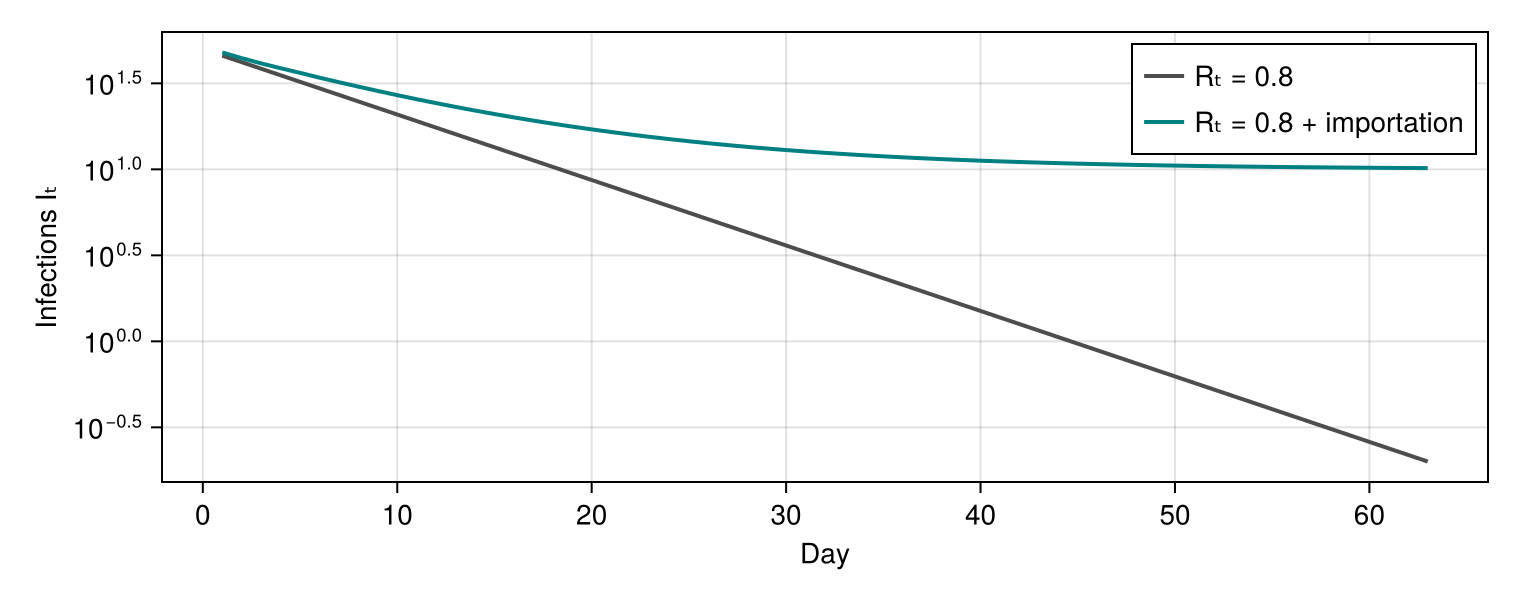

Fitting a model with modifiers

Modifiers are part of the model, so a model carrying them is fitted exactly like any other. An ImportedCases rate is a prior slot, so it is estimated rather than assumed: here it is a single unknown constant on the log scale, drawn once before the renewal recursion runs. We fit that model to the reported cases simulated above. The reproduction number is still held at its simulated value, so the importation rate is what is being learned; with free as well the two compete to explain the same growth and the fit is much less sharp. The unobserved days at the start are missing entries of y_obs, and are sampled rather than conditioned on.

model = IDModel(
    renewal(SusceptibleDepletion(pop_size),
        ImportedCases(Normal(0.0, 1.0))),
    obs)
y_obs = sims.seeded.generated_y_t
chain = sample(as_turing_model(model, y_obs, n),
    NUTS(0.95; adtype = AutoMooncake(; config = nothing)), 250;
    progress = false)

┌ Info: Found initial step size
└   ϵ = 0.025

The rate is namespaced by the modifier's position on the renewal step, so several modifiers carrying priors can never collide. Exponentiating the draws puts it back on the scale of infections per day, where the true value was two.

import_draws = exp.(vec(chain[@varname(modifier_2.import_rates)]))
(posterior = round.(quantile(import_draws, [0.05, 0.5, 0.95]), digits = 2),
    truth = 2.0)

(posterior = [1.75, 2.05, 2.4], truth = 2.0)

The posterior predictive then tracks the simulated series.

pred = predict(as_turing_model(model, fill(missing, n), n), chain)
y_draws(i) = Float64.(vec(pred[@varname(y_t[i])]))
quantiles(i) = quantile(y_draws(i), [0.05, 0.5, 0.95])
bands = reduce(hcat, map(quantiles, obs_days))

fig3 = Figure(; size = (760, 300))
ax4 = Axis(fig3[1, 1]; xlabel = "Day", ylabel = "Reported cases",
    yscale = log10)
band!(ax4, obs_days, max.(bands[1, :], 1), max.(bands[3, :], 1);
    color = (:teal, 0.25))
lines!(ax4, obs_days, max.(bands[2, :], 1); color = :teal, linewidth = 2,
    label = "posterior predictive")
scatter!(ax4, obs_days, max.(y_obs[obs_days], 1); color = :black,
    markersize = 7, label = "simulated")
axislegend(ax4; position = :lt)
fig3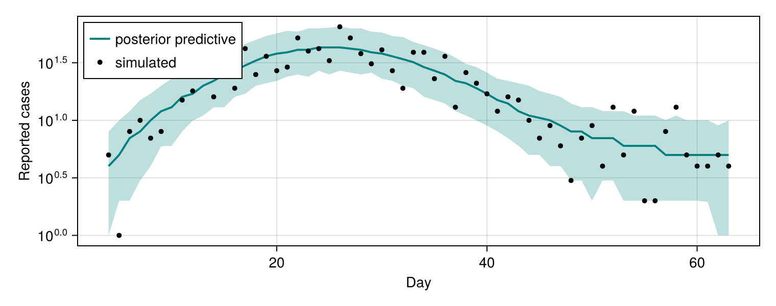

Summary

Both extensions are one positional argument on Renewal, and neither changes the observation model, the latent process, or the fitting code. Each draws whatever it does not know through the same seam every other component uses, so the importation rate can equally be a fixed constant, an unknown constant, or a time-varying process such as a RandomWalk — in every case the prior is on the log scale, like every other unknown positive quantity here.