Multiple observation streams: cases, deaths, and strata
Real-time surveillance rarely watches an epidemic through a single lens. The same infections surface as reported cases, hospital admissions, deaths, and often each of these split by age, region, or variant. These streams share one underlying infection process but differ in their reporting delay, ascertainment, and noise [4]. Fitting them jointly, one infection trajectory and several observation streams, propagates uncertainty correctly and lets a sparse stream (deaths) borrow strength from a dense one (cases).
This tutorial uses one construct, Split, for every multi-stream shape. Split observes the expected series arriving at the point where it sits in the pipeline through several named streams, so where you place it chooses the composition.
Parallel, placed high on infections. Every stream observes the same
, cases and deaths each a delayed, ascertained fraction of . Cascade, placed low after a shared layer. A later stream is observed downstream of an earlier one, deaths as a delayed fraction of the expected reported cases.
Strata, one stream per data-defined group such as an age band.
How Split threads streams
Every observation model in the package returns the uniform pair (; y_t, expected), the sampled observations y_t and the pre-error expected series the error was scored against. Exposing expected is what lets Split do all three shapes with one mechanism. Split feeds each stream the expected series reaching it, and because Split is itself an observation model a shared modifier can run before it. Split((cases = …, deaths = …)) on its own splits infections (parallel). LatentDelay(Split((cases = …, deaths = …)), pmf) applies a common delay first and then splits, so a stream nested inside another stream's pipeline sits downstream of it (cascade).
The threaded quantity is the expected, not the realised, series
A downstream stream reads its upstream stream's expected (pre-error) series, never its realised, sampled counts. So a cascade threads the mean reported cases into deaths, not a noisy draw. The case where an observation depends on another stream's realised observation is not covered here and is out of scope for now.
Split also prefixes each stream's sampled variables with the stream name automatically, so the streams stay distinct without any manual prefix layer.
Parallel: cases and deaths from shared infections
We drive the streams with a renewal infection process, exactly as in the renewal tutorial, and observe it through two pipelines. Cases are a short-delay, high-ascertainment negative-binomial stream. Deaths are a long-delay stream whose ascertainment, the infection-fatality ratio, is itself estimated. Each stream is a full observation model, so its ascertainment can be a fixed fraction or, as here, a latent Intercept model with a prior.
using ComposableTuringIDModels, Distributions, Random, Turing, Mooncake
using ADTypes: AutoMooncake
using Accessors
Random.seed!(1234)

latent = AR(
    damp = [truncated(Normal(0.8, 0.05), 0, 1),
        truncated(Normal(0.1, 0.05), 0, 1)],
    init = [Normal(0.0, 0.2), Normal(0.0, 0.2)],
    ϵ_t = HierarchicalNormal(std = HalfNormal(0.1)))
renewal = Renewal(; generation_time = Gamma(6.5, 0.62),
    rt = latent, initialisation = Normal(log(100.0), 0.1))

cases = LatentDelay(
    Ascertainment(NegativeBinomialError(cluster_factor = HalfNormal(0.1)),
        FixedIntercept(log(0.6))),                     # ~60% case ascertainment
    LogNormal(1.6, 0.5))                                # short infection→report delay
deaths = @set cases.model.latent_model = Intercept(Normal(log(0.015), 0.25))  # ~1.5% IFR
deaths = @set deaths.delay = LogNormal(2.8, 0.4)    # long infection→death delay

parallel = Split((cases = cases, deaths = deaths))
Split
├─ cases: LatentDelay
│ └─ model: Ascertainment
│ ├─ model: NegativeBinomialError
│ └─ latent: PrefixLatentModel
│ └─ model: FixedIntercept
└─ deaths: LatentDelay
└─ model: Ascertainment
├─ model: NegativeBinomialError
└─ latent: PrefixLatentModel
└─ model: InterceptA multi-stream model is assembled exactly like a single-stream one.
model = IDModel(renewal, parallel)IDModel
├─ infection: Renewal
│ └─ rt: AR
│ └─ ϵ_t: HierarchicalNormal
└─ observation: Split
├─ cases: LatentDelay
│ └─ model: Ascertainment
│ ├─ model: NegativeBinomialError
│ └─ latent: PrefixLatentModel
│ └─ model: FixedIntercept
└─ deaths: LatentDelay
└─ model: Ascertainment
├─ model: NegativeBinomialError
└─ latent: PrefixLatentModel
└─ model: InterceptPassing missing data simulates a synthetic outbreak. The per-stream data contract is a NamedTuple keyed by stream name, and the returned generated_y_t is a NamedTuple of the two simulated series.
n = 70
sim = as_turing_model(model, (cases = missing, deaths = missing), n)()
y = sim.generated_y_t
(total_cases = sum(y.cases), total_deaths = sum(y.deaths),
    n_cases = length(y.cases), n_deaths = length(y.deaths))
(total_cases = 16020, total_deaths = 310, n_cases = 96, n_deaths = 70)The two series come back at different lengths. One infection series serves both streams, so it is long enough for the deeper infection→death delay, and the shorter infection→report delay leaves the cases stream with expected values for earlier days too. Both are scored. Pass each stream the observations it has, and data_requirements reports the two lengths before the model is built.
Fitting conditions on both streams at once. We draw two chains in parallel with MCMCThreads(), matching the other tutorials, and differentiate with Mooncake, the recommended backend for this package (see Automatic differentiation backend).
ydata = (cases = y.cases, deaths = y.deaths)
posterior = as_turing_model(model, ydata, n)
chain = sample(
    posterior, NUTS(0.95; adtype = AutoMooncake(; config = nothing)),
    MCMCThreads(), 250, 2; progress = false)
┌ Info: Found initial step size
└ ϵ = 0.0125
┌ Info: Found initial step size
└ ϵ = 0.003125
┌ Warning: There were 11 divergent transitions. Consider reparameterising your model or using a smaller step size. For adaptive samplers such as NUTS and HMCDA, consider increasing `target_accept`.
└ @ Turing.Inference ~/.julia/packages/Turing/4sXd9/src/mcmc/hmc.jl:483
┌ Warning: There were 4 divergent transitions. Consider reparameterising your model or using a smaller step size. For adaptive samplers such as NUTS and HMCDA, consider increasing `target_accept`.
└ @ Turing.Inference ~/.julia/packages/Turing/4sXd9/src/mcmc/hmc.jl:483
┌ Warning: There were 15 divergent transitions. Consider reparameterising your model or using a smaller step size. For adaptive samplers such as NUTS and HMCDA, consider increasing `target_accept`.
└ @ Turing.Inference ~/.julia/packages/Turing/4sXd9/src/mcmc/hmc.jl:483The two streams keep their own overdispersion parameters, prefixed by Split as cases.cluster_factor and deaths.cluster_factor, while sharing the one infection trajectory. The deaths stream's estimated IFR intercept (deaths.Ascertainment.intercept) is recovered alongside them. The dense case stream pins the shared
using MCMCChains
summarystats(chain)╭─FlexiSummary (9 statistics) ─────────────────────────────────────────────────╮
│ iter collapsed │
│ chain collapsed │
│ ↓ stat = [mean, std, mcse, ess_bulk, ess_tail, rhat, q5, q50, q95] │
│ │
│ Parameters (118) ── AbstractPPL.VarName │
│ Float64 init[1], init[2], damp[1], damp[2], std, ϵ_t[1], ϵ_t[2], ϵ_t[3], │
│ ϵ_t[4], ϵ_t[5], ϵ_t[6], ϵ_t[7], ϵ_t[8], ϵ_t[9], ϵ_t[10], ϵ_t[11], │
│ ϵ_t[12], ϵ_t[13], ϵ_t[14], ϵ_t[15], ϵ_t[16], ϵ_t[17], ϵ_t[18], │
│ ϵ_t[19], ϵ_t[20], ϵ_t[21], ϵ_t[22], ϵ_t[23], ϵ_t[24], ϵ_t[25], │
│ ϵ_t[26], ϵ_t[27], ϵ_t[28], ϵ_t[29], ϵ_t[30], ϵ_t[31], ϵ_t[32], │
│ ϵ_t[33], ϵ_t[34], ϵ_t[35], ϵ_t[36], ϵ_t[37], ϵ_t[38], ϵ_t[39], │
│ ϵ_t[40], ϵ_t[41], ϵ_t[42], ϵ_t[43], ϵ_t[44], ϵ_t[45], ϵ_t[46], │
│ ϵ_t[47], ϵ_t[48], ϵ_t[49], ϵ_t[50], ϵ_t[51], ϵ_t[52], ϵ_t[53], │
│ ϵ_t[54], ϵ_t[55], ϵ_t[56], ϵ_t[57], ϵ_t[58], ϵ_t[59], ϵ_t[60], │
│ ϵ_t[61], ϵ_t[62], ϵ_t[63], ϵ_t[64], ϵ_t[65], ϵ_t[66], ϵ_t[67], │
│ ϵ_t[68], ϵ_t[69], ϵ_t[70], ϵ_t[71], ϵ_t[72], ϵ_t[73], ϵ_t[74], │
│ ϵ_t[75], ϵ_t[76], ϵ_t[77], ϵ_t[78], ϵ_t[79], ϵ_t[80], ϵ_t[81], │
│ ϵ_t[82], ϵ_t[83], ϵ_t[84], ϵ_t[85], ϵ_t[86], ϵ_t[87], ϵ_t[88], │
│ ϵ_t[89], ϵ_t[90], ϵ_t[91], ϵ_t[92], ϵ_t[93], ϵ_t[94], ϵ_t[95], │
│ ϵ_t[96], ϵ_t[97], ϵ_t[98], ϵ_t[99], ϵ_t[100], ϵ_t[101], ϵ_t[102], │
│ ϵ_t[103], ϵ_t[104], ϵ_t[105], ϵ_t[106], ϵ_t[107], ϵ_t[108], │
│ ϵ_t[109], init_incidence, cases.cluster_factor, │
│ deaths.Ascertainment.intercept, deaths.cluster_factor │
│ │
│ Extras (14) │
│ Float64 n_steps, is_accept, acceptance_rate, log_density, │
│ hamiltonian_energy, hamiltonian_energy_error, │
│ max_hamiltonian_energy_error, tree_depth, numerical_error, │
│ step_size, nom_step_size, logprior, loglikelihood, logjoint │
│ │
│ Summary │
│ param mean std mcse ess_bulk ess_tail rhat … │
│ init[1] -0.0227 0.2038 0.0084 577.7401 275.8699 1.0093 … │
│ init[2] 0.2929 0.1546 0.0074 446.6991 365.8559 0.9984 … │
│ damp[1] 0.7867 0.0441 0.0019 564.7188 307.7958 0.9989 … │
│ damp[2] 0.0940 0.0400 0.0015 641.7088 261.9963 1.0016 … │
│ std 0.0649 0.0249 0.0015 274.3217 393.9547 1.0018 … │
│ ϵ_t[1] 0.4318 0.9690 0.0372 672.6815 277.5190 1.0003 … │
│ ϵ_t[2] 0.4195 0.8919 0.0331 753.5502 322.1994 1.0013 … │
│ ϵ_t[3] 0.3559 1.0134 0.0464 465.5643 203.6652 1.0057 … │
│ ϵ_t[4] 0.3860 1.0400 0.0462 510.0710 269.8742 1.0053 … │
│ ϵ_t[5] 0.3324 0.9266 0.0383 588.9175 384.3815 0.9985 … │
│ ϵ_t[6] 0.3639 0.8827 0.0386 524.4017 406.2668 0.9992 … │
│ ϵ_t[7] 0.3275 0.9881 0.0387 658.5709 403.9435 1.0002 … │
│ ϵ_t[8] 0.2949 1.0141 0.0364 777.0423 436.0858 0.9988 … │
│ ϵ_t[9] 0.2080 1.0101 0.0416 578.5732 333.2991 1.0049 … │
│ ϵ_t[10] 0.2214 1.0365 0.0363 818.2152 333.4376 1.0007 … │
│ ϵ_t[11] 0.1460 0.8948 0.0321 782.4315 406.3628 0.9982 … │
│ ϵ_t[12] 0.1219 0.9868 0.0344 823.3165 336.4685 1.0001 … │
│ ϵ_t[13] 0.0230 0.9913 0.0390 643.3632 370.0785 1.0050 … │
│ ϵ_t[14] -0.0962 1.0011 0.0406 604.7159 378.4095 0.9984 … │
│ ϵ_t[15] -0.1309 1.0172 0.0389 694.8572 328.4725 1.0033 … │
│ ϵ_t[16] -0.1646 0.9237 0.0386 578.3658 436.0858 1.0059 … │
│ ϵ_t[17] -0.1955 1.0027 0.0450 510.2610 333.2991 1.0098 … │
│ ϵ_t[18] -0.2094 1.0217 0.0385 699.4265 298.5696 1.0000 … │
│ ϵ_t[19] -0.2338 0.9273 0.0350 710.3885 340.8394 1.0006 … │
│ ϵ_t[20] -0.2333 1.0491 0.0391 736.4619 391.6587 1.0009 … │
│ ϵ_t[21] -0.3088 0.9272 0.0322 853.1118 253.9588 1.0154 … │
│ ϵ_t[22] -0.2612 0.9904 0.0378 693.1323 323.5581 1.0008 … │
│ ϵ_t[23] -0.2116 1.0531 0.0377 790.0310 375.4466 0.9990 … │
│ ϵ_t[24] -0.2640 0.9690 0.0417 539.3703 238.8544 1.0043 … │
│ ϵ_t[25] -0.2495 0.9859 0.0394 622.5224 357.1907 0.9992 … │
│ ϵ_t[26] -0.2470 0.9535 0.0379 624.7843 299.6594 1.0028 … │
│ ϵ_t[27] -0.2598 1.0302 0.0391 687.2562 269.0382 0.9992 … │
│ ϵ_t[28] -0.2733 1.0024 0.0403 619.6061 369.3744 0.9983 … │
│ ϵ_t[29] -0.3461 1.0513 0.0402 684.7753 133.2257 0.9999 … │
│ ϵ_t[30] -0.2540 0.9660 0.0406 573.3123 280.3587 1.0002 … │
│ ϵ_t[31] -0.3567 0.9432 0.0383 585.1675 324.3197 0.9981 … │
│ ϵ_t[32] -0.3702 1.0248 0.0421 596.7918 201.8018 1.0053 … │
│ ϵ_t[33] -0.4402 1.0328 0.0420 610.7330 257.6662 0.9985 … │
│ ϵ_t[34] -0.3411 0.9582 0.0421 517.7666 392.9141 1.0010 … │
│ ϵ_t[35] -0.3118 0.9640 0.0408 554.9526 351.7456 1.0028 … │
│ ϵ_t[36] -0.2215 0.9155 0.0387 555.5267 381.4196 1.0039 … │
│ ϵ_t[37] -0.1785 0.9132 0.0326 775.8198 415.4768 0.9980 … │
│ ϵ_t[38] -0.0538 0.9250 0.0352 692.9295 269.8338 1.0027 … │
│ ϵ_t[39] 0.0033 0.9787 0.0432 527.9000 396.9296 1.0296 … │
│ ϵ_t[40] 0.0393 1.0007 0.0388 663.4300 289.9710 1.0020 … │
│ ϵ_t[41] 0.2008 0.9736 0.0380 673.5719 352.1938 1.0007 … │
│ ϵ_t[42] 0.2509 0.9721 0.0396 623.6345 327.3183 1.0280 … │
│ ϵ_t[43] 0.2131 0.9100 0.0370 605.6418 368.7272 1.0030 … │
│ ϵ_t[44] 0.1906 1.0525 0.0428 617.1643 349.8738 1.0002 … │
│ ϵ_t[45] 0.1714 0.9066 0.0393 513.1758 316.1157 1.0107 … │
│ ϵ_t[46] 0.1906 0.9865 0.0407 593.0322 281.8821 0.9984 … │
│ ϵ_t[47] 0.1911 0.9718 0.0421 549.3014 332.4821 1.0005 … │
│ ϵ_t[48] 0.3211 0.9946 0.0436 528.9946 270.9625 1.0048 … │
│ ϵ_t[49] 0.2689 0.9641 0.0414 538.2452 301.1264 1.0011 … │
│ ϵ_t[50] 0.2262 0.9408 0.0389 592.7407 329.7230 1.0268 … │
│ ϵ_t[51] 0.1309 1.0006 0.0407 598.5578 325.4780 1.0032 … │
│ ϵ_t[52] 0.1127 0.8803 0.0337 665.0036 283.6091 1.0001 … │
│ ϵ_t[53] 0.0117 0.9669 0.0348 758.1336 347.5764 0.9993 … │
│ ϵ_t[54] 0.0468 0.9802 0.0417 554.6650 318.0299 0.9995 … │
│ ϵ_t[55] 0.1109 0.9585 0.0396 591.1360 348.6718 1.0142 … │
│ ϵ_t[56] 0.0997 0.9675 0.0356 715.4849 374.6171 0.9986 … │
│ ϵ_t[57] 0.1545 1.0156 0.0406 650.7022 374.3784 1.0014 … │
│ ϵ_t[58] 0.1381 0.8701 0.0409 450.8362 332.4821 0.9997 … │
│ ϵ_t[59] 0.1132 0.9449 0.0345 765.0168 349.5964 0.9982 … │
│ ϵ_t[60] -0.0198 0.9997 0.0415 583.2449 156.3896 1.0030 … │
│ ϵ_t[61] -0.1149 0.9564 0.0373 707.3272 438.9538 0.9985 … │
│ ϵ_t[62] -0.0381 1.0830 0.0506 464.8802 282.3512 1.0017 … │
│ ϵ_t[63] -0.1346 0.9266 0.0406 532.6758 335.5995 1.0062 … │
│ ϵ_t[64] -0.0556 1.0149 0.0404 655.6024 282.4193 0.9988 … │
│ ϵ_t[65] -0.0128 0.8973 0.0364 625.6683 325.0995 0.9984 … │
│ ϵ_t[66] 0.0110 0.9909 0.0401 611.6525 364.0645 1.0001 … │
│ ϵ_t[67] 0.0496 0.9465 0.0367 710.0745 293.0490 1.0151 … │
│ ϵ_t[68] 0.3455 0.9260 0.0394 574.3925 270.2551 1.0024 … │
│ ϵ_t[69] 0.3853 0.8874 0.0315 798.0799 438.4716 0.9986 … │
│ ϵ_t[70] 0.4219 0.9202 0.0362 639.7260 259.6722 1.0019 … │
│ ϵ_t[71] 0.4904 0.8765 0.0328 725.5820 391.1356 0.9995 … │
│ ϵ_t[72] 0.4664 0.8604 0.0344 611.8375 305.4884 1.0037 … │
│ ϵ_t[73] 0.4188 0.9222 0.0362 656.1812 437.0197 0.9983 … │
│ ϵ_t[74] 0.4011 0.8972 0.0380 557.7766 396.5658 1.0027 … │
│ ϵ_t[75] 0.2461 0.9013 0.0413 477.4009 348.3878 0.9996 … │
│ ϵ_t[76] 0.0820 0.9627 0.0382 655.1299 382.4154 1.0010 … │
│ ϵ_t[77] 0.1529 0.9528 0.0364 684.9790 412.5829 1.0031 … │
│ ϵ_t[78] 0.1980 0.9742 0.0449 466.2994 333.2991 1.0001 … │
│ ϵ_t[79] 0.3090 0.9763 0.0366 693.0821 323.0863 1.0030 … │
│ ϵ_t[80] 0.3059 1.0319 0.0386 686.3459 312.6279 0.9990 … │
│ ϵ_t[81] 0.3402 0.9879 0.0429 554.5445 279.2898 1.0033 … │
│ ϵ_t[82] 0.4195 1.0210 0.0383 715.1491 353.1196 1.0002 … │
│ ϵ_t[83] 0.4060 0.9306 0.0349 695.6447 349.0795 1.0004 … │
│ ϵ_t[84] 0.3460 0.8990 0.0406 493.7962 325.4343 1.0006 … │
│ ϵ_t[85] 0.2549 0.9418 0.0330 829.7342 277.5116 1.0087 … │
│ ϵ_t[86] 0.2070 0.9492 0.0379 609.9918 229.2191 0.9989 … │
│ ϵ_t[87] 0.1331 0.9735 0.0378 668.4032 341.0097 0.9984 … │
│ ϵ_t[88] 0.0183 1.0290 0.0380 728.4579 301.3976 0.9996 … │
│ ϵ_t[89] -0.1736 0.9450 0.0449 433.0332 281.8821 0.9996 … │
│ ϵ_t[90] -0.1939 0.9449 0.0398 569.0826 392.5833 1.0001 … │
│ ϵ_t[91] -0.2734 0.9886 0.0377 703.5732 279.0983 1.0058 … │
│ ϵ_t[92] -0.3598 0.9575 0.0334 816.8809 355.0748 1.0018 … │
│ ϵ_t[93] -0.3804 0.9444 0.0382 608.2393 375.4466 1.0011 … │
│ ϵ_t[94] -0.4530 0.8887 0.0368 579.7899 348.7163 1.0035 … │
│ ϵ_t[95] -0.3398 0.9285 0.0363 652.7472 369.1484 1.0025 … │
│ ϵ_t[96] -0.2473 0.9899 0.0409 577.5795 306.2890 0.9992 … │
│ ϵ_t[97] -0.3072 0.9744 0.0394 612.4914 363.5804 1.0047 … │
│ ϵ_t[98] -0.1777 0.9391 0.0372 604.4122 368.0397 1.0003 … │
│ ϵ_t[99] -0.2208 1.0107 0.0339 903.0983 425.5089 1.0041 … │
│ ϵ_t[100] -0.1196 1.0247 0.0450 529.0498 237.9373 1.0084 … │
│ ϵ_t[101] -0.0210 0.9731 0.0386 628.4939 333.2991 1.0025 … │
│ ϵ_t[102] 0.0351 0.9241 0.0419 491.4158 353.6635 1.0113 … │
│ ϵ_t[103] -0.0090 1.0608 0.0407 683.2922 361.0341 1.0083 … │
│ ϵ_t[104] -0.0185 0.9269 0.0397 548.8375 333.2991 1.0031 … │
│ ϵ_t[105] -0.0295 1.0696 0.0421 649.0879 278.3590 1.0015 … │
│ ϵ_t[106] -0.0134 1.0070 0.0414 582.9592 302.6508 0.9988 … │
│ ϵ_t[107] -0.0987 0.9684 0.0341 806.9344 313.0627 1.0023 … │
│ ϵ_t[108] -0.0089 0.9952 0.0405 618.9399 301.1735 1.0148 … │
│ ϵ_t[109] 0.0155 0.9951 0.0396 620.8156 333.2991 0.9992 … │
│ init_incide… 4.6471 0.0951 0.0044 476.2310 387.1280 1.0022 … │
│ cases.clust… 0.1882 0.0176 0.0009 423.0800 404.8045 1.0034 … │
│ deaths.Asce… -4.0873 0.0625 0.0028 506.5228 349.8661 0.9986 … │
│ deaths.clus… 0.1206 0.0768 0.0040 240.4941 142.8993 1.0022 … │
╰──────────────────────────────────────────────────────────────────────────────╯Summary statistics confirm the parameters converged, but they do not show whether the fit actually tracks the two simulated series. Posterior-predictive draws from the same fitted chain, plotted against the simulated counts, close that loop. The helpers below turn a time × draws matrix into 50% and 95% credible bands and draw a median line with ribbons. predictive_bands walks a named stream's per-index sampled y_t, filling any index a stream's delay leaves unscored with missing.
Split prefixes each stream's y_t, so predictive_bands reads cases.y_t[i] and deaths.y_t[i] off the predict chain, the prefixed equivalent of the bare y_t[i] the renewal tutorial reads from a single-stream model.
missmodel = as_turing_model(model, (cases = missing, deaths = missing), n)
pred = predict(missmodel, chain)

# Each stream is scored over its own expected series, so read its bands at its
# own length. Both end on the same day, so a shared day axis ending at `n`
# right-aligns them the way the model does.
cases_days = (n - length(y.cases) + 1):n
deaths_days = (n - length(y.deaths) + 1):n
cases_bands = predictive_bands(
    pred, length(y.cases), i -> @varname(cases.y_t[i]))
deaths_bands = predictive_bands(
    pred, length(y.deaths), i -> @varname(deaths.y_t[i]))

fig = Figure(; size = (760, 620))
ax1 = Axis(fig[1, 1]; ylabel = "Cases")
ci_ribbon!(ax1, cases_days, cases_bands; color = :teal,
    label = "posterior predictive")
scatter!(ax1, cases_days, y.cases; color = :black, markersize = 6,
    label = "simulated")
axislegend(ax1; position = :lt)
ax2 = Axis(fig[2, 1]; xlabel = "Day", ylabel = "Deaths")
ci_ribbon!(ax2, deaths_days, deaths_bands; color = :firebrick,
    label = "posterior predictive")
scatter!(ax2, deaths_days, y.deaths; color = :black, markersize = 6,
    label = "simulated")
axislegend(ax2; position = :lt)
fig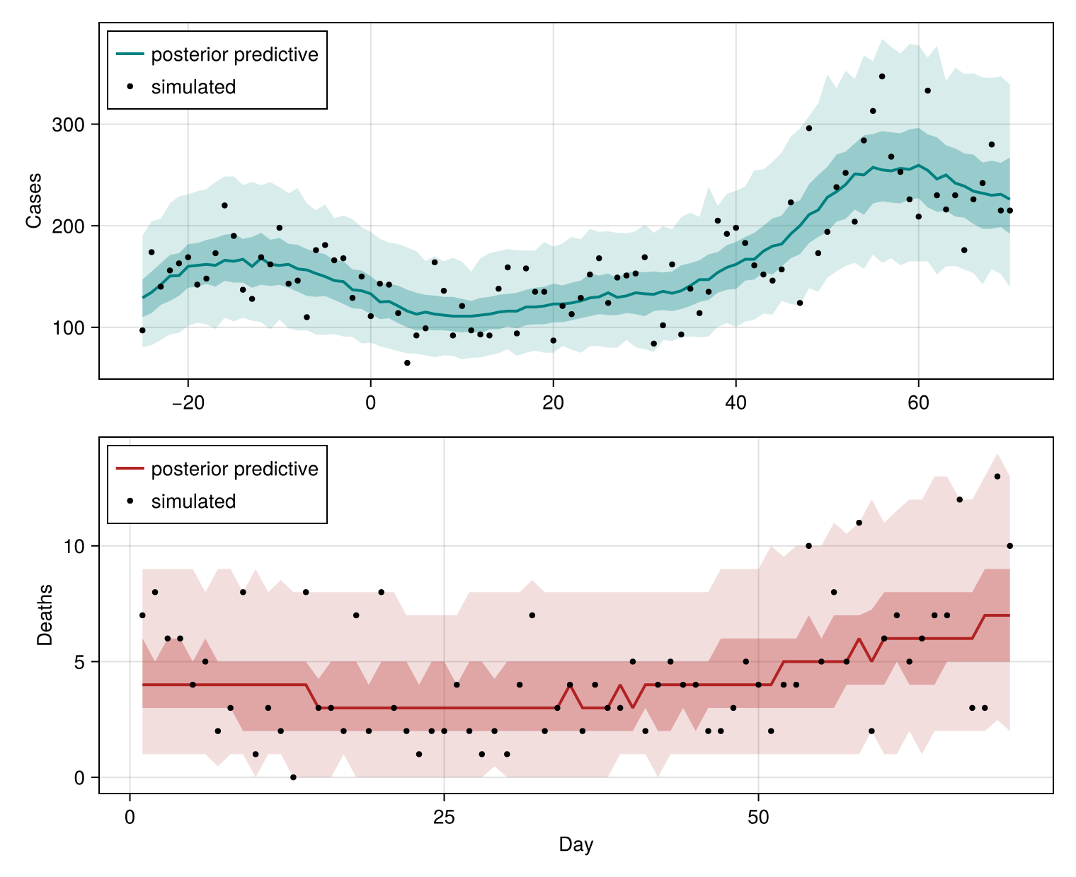
The band covers the simulated series on almost every day for both streams, and both medians track the outbreak's rise and fall rather than sitting flat at the mean. The sparser death series (82 simulated deaths against 6576 cases over the same 70 days) still recovers. Its band is visibly wider, but it moves with the same underlying trajectory rather than needing its own signal to do so.
Cascade: deaths downstream of reported cases
In the parallel model, cases and deaths both branch off infections, so a reporting artefact in the case series (a weekend dip, an ascertainment change) does not touch deaths. Sometimes we want the opposite, deaths modelled as a delayed fraction of the reported cases, so whatever is reflected in cases propagates into deaths. That is a cascade Split placed lower in the stack. Share the infection→case-report delay, then split.
cascade = LatentDelay(                                   # infection→case delay
    Split((
        cases = NegativeBinomialError(cluster_factor = HalfNormal(0.1)),
        deaths = LatentDelay(                            # case→death delay
            Ascertainment(NegativeBinomialError(cluster_factor = HalfNormal(0.1)),
                FixedIntercept(log(0.02))),
            LogNormal(2.2, 0.3)))),
    LogNormal(1.6, 0.5))
LatentDelay
└─ model: Split
├─ cases: NegativeBinomialError
└─ deaths: LatentDelay
└─ model: Ascertainment
├─ model: NegativeBinomialError
└─ latent: PrefixLatentModel
└─ model: FixedInterceptThe deaths stream's expected input is the delayed-and-ascertained expected cases rather than the raw infections, so it is both scaled by the fatality fraction and shortened by the case delay.
cascade_model = IDModel(renewal, cascade)
cas = as_turing_model(cascade_model, (cases = missing, deaths = missing), n)()
(cases_expected = length(cas.expected_y_t.cases),
    deaths_expected = length(cas.expected_y_t.deaths),
    deaths_per_case = round(
        sum(cas.expected_y_t.deaths) / sum(cas.expected_y_t.cases), digits = 3))
(cases_expected = 87, deaths_expected = 70, deaths_per_case = 0.018)Strata: one stream per age band
A stratified stream, one observation series per age band, region, or variant, is again the same construct, here composed with the renewal infection process and observed through one named stream per band. Each band is a full observation model, so its delay and ascertainment can differ, and its parameters are namespaced by the band name.
strata_obs = Split((
    young = LatentDelay(
        Ascertainment(NegativeBinomialError(cluster_factor = HalfNormal(0.1)),
            FixedIntercept(log(0.7))), LogNormal(1.5, 0.4)),
    old = LatentDelay(
        Ascertainment(NegativeBinomialError(cluster_factor = HalfNormal(0.1)),
            FixedIntercept(log(0.4))), LogNormal(1.8, 0.4))))
strata_model = IDModel(renewal, strata_obs)
strata_sim = as_turing_model(
    strata_model, (young = missing, old = missing), n)().generated_y_t
map(s -> sum(skipmissing(s)), strata_sim)                # totals per band
(young = 1085, old = 583)The streams above each observe the same infections. When the streams instead draw on a weighted mix of infections, one band, another band, and a summed total, the same Split carries an observation-strata × infection-strata weight matrix, and a single template model is replicated once per data stream. Split(template, W) projects the infection series reaching it through W, so it composes inside an IDModel like any other observation model. The infections come from the modelled process, not a hand-built series. One weight matrix covers the one-to-one (an identity map), many-to-one (an aggregation row summing infection strata into one stream), and many-to-many (a general matrix) infection → observation cases.
Here the renewal process supplies one infection stratum, and W maps it onto a young band, an old band, and their total.
W = reshape([0.7, 0.3, 1.0], 3, 1)                  # young, old, and their total
weighted = Split(LatentDelay(PoissonError(), LogNormal(1.6, 0.5)), W)
weighted_model = IDModel(renewal, weighted)
age = as_turing_model(
    weighted_model, (young = missing, old = missing, total = missing), n)()
map(s -> sum(skipmissing(s)), age.generated_y_t)         # simulated total per band
(young = 407386, old = 173726, total = 580933)The aggregate total stream sees the summed expected infections of both bands, so its expected series is exactly young .+ old.
Simulating checks that the forward map runs. It does not check that a many-to-one W is actually recoverable from data. Fitting weighted_model to its own simulated streams answers that. The fit conditions on young, old, and the aggregate total together, exactly as Split conditions on any other named streams.
weighted_data = (young = age.generated_y_t.young, old = age.generated_y_t.old,
    total = age.generated_y_t.total)
weighted_posterior = as_turing_model(weighted_model, weighted_data, n)
weighted_chain = sample(
    weighted_posterior, NUTS(0.95; adtype = AutoMooncake(; config = nothing)),
    MCMCThreads(), 250, 2; progress = false)
┌ Info: Found initial step size
└ ϵ = 0.0001953125
┌ Info: Found initial step size
└ ϵ = 6.462348535570529e-28young, old, and total are not three independent counts. total is exactly young + old, so all three read the same one-stratum
summarystats(weighted_chain)╭─FlexiSummary (9 statistics) ─────────────────────────────────────────────────╮
│ iter collapsed │
│ chain collapsed │
│ ↓ stat = [mean, std, mcse, ess_bulk, ess_tail, rhat, q5, q50, q95] │
│ │
│ Parameters (89) ── AbstractPPL.VarName │
│ Float64 init[1], init[2], damp[1], damp[2], std, ϵ_t[1], ϵ_t[2], ϵ_t[3], │
│ ϵ_t[4], ϵ_t[5], ϵ_t[6], ϵ_t[7], ϵ_t[8], ϵ_t[9], ϵ_t[10], ϵ_t[11], │
│ ϵ_t[12], ϵ_t[13], ϵ_t[14], ϵ_t[15], ϵ_t[16], ϵ_t[17], ϵ_t[18], │
│ ϵ_t[19], ϵ_t[20], ϵ_t[21], ϵ_t[22], ϵ_t[23], ϵ_t[24], ϵ_t[25], │
│ ϵ_t[26], ϵ_t[27], ϵ_t[28], ϵ_t[29], ϵ_t[30], ϵ_t[31], ϵ_t[32], │
│ ϵ_t[33], ϵ_t[34], ϵ_t[35], ϵ_t[36], ϵ_t[37], ϵ_t[38], ϵ_t[39], │
│ ϵ_t[40], ϵ_t[41], ϵ_t[42], ϵ_t[43], ϵ_t[44], ϵ_t[45], ϵ_t[46], │
│ ϵ_t[47], ϵ_t[48], ϵ_t[49], ϵ_t[50], ϵ_t[51], ϵ_t[52], ϵ_t[53], │
│ ϵ_t[54], ϵ_t[55], ϵ_t[56], ϵ_t[57], ϵ_t[58], ϵ_t[59], ϵ_t[60], │
│ ϵ_t[61], ϵ_t[62], ϵ_t[63], ϵ_t[64], ϵ_t[65], ϵ_t[66], ϵ_t[67], │
│ ϵ_t[68], ϵ_t[69], ϵ_t[70], ϵ_t[71], ϵ_t[72], ϵ_t[73], ϵ_t[74], │
│ ϵ_t[75], ϵ_t[76], ϵ_t[77], ϵ_t[78], ϵ_t[79], ϵ_t[80], ϵ_t[81], │
│ ϵ_t[82], ϵ_t[83], init_incidence │
│ │
│ Extras (14) │
│ Float64 n_steps, is_accept, acceptance_rate, log_density, │
│ hamiltonian_energy, hamiltonian_energy_error, │
│ max_hamiltonian_energy_error, tree_depth, numerical_error, │
│ step_size, nom_step_size, logprior, loglikelihood, logjoint │
│ │
│ Summary │
│ param mean std mcse ess_bulk ess_tail rhat … │
│ init[1] 0.2714 1.5442 1.5318 1.3139 10.8746 2.1263 … │
│ init[2] 0.7378 0.1211 0.0447 5.9304 10.8746 2.1263 … │
│ damp[1] 0.4971 0.3444 0.3415 1.3340 10.8746 2.1263 … │
│ damp[2] 0.3020 0.1919 0.1904 1.3182 10.8746 2.1263 … │
│ std 1.8343 1.6034 1.5903 1.3175 10.8746 2.1263 … │
│ ϵ_t[1] 1.3423 0.2155 0.2127 1.3105 10.8746 2.1263 … │
│ ϵ_t[2] -1.1324 0.2111 0.2090 1.3166 10.8746 2.1263 … │
│ ϵ_t[3] -1.7341 0.0886 0.0868 1.3185 10.8746 2.1263 … │
│ ϵ_t[4] -0.3298 1.4398 1.4282 1.3286 10.8746 2.1263 … │
│ ϵ_t[5] 0.7161 0.0635 0.0614 1.3206 10.8746 2.1263 … │
│ ϵ_t[6] 0.3518 0.4763 0.4723 1.3258 10.8746 2.1263 … │
│ ϵ_t[7] -1.4885 0.3696 0.3663 1.3166 10.8746 2.1263 … │
│ ϵ_t[8] -0.0552 0.2998 0.2970 1.3188 10.8746 2.1263 … │
│ ϵ_t[9] 0.1008 0.7011 0.6952 1.3279 10.8746 2.1263 … │
│ ϵ_t[10] 1.0070 0.0756 0.0706 1.3258 10.8746 2.1263 … │
│ ϵ_t[11] 0.1191 1.0843 1.0753 1.3258 10.8746 2.1263 … │
│ ϵ_t[12] -0.2545 0.7242 0.7178 1.3253 10.8746 2.1263 … │
│ ϵ_t[13] 1.3870 0.5062 0.5012 1.3212 10.8746 2.1263 … │
│ ϵ_t[14] -0.6587 1.3447 1.3334 1.3252 10.8746 2.1263 … │
│ ϵ_t[15] -0.5595 0.3866 0.3823 1.3257 10.8746 2.1263 … │
│ ϵ_t[16] 0.2525 0.2586 0.2531 1.3250 10.8746 2.1263 … │
│ ϵ_t[17] 0.8848 0.0524 0.0217 5.8354 12.2368 2.1263 … │
│ ϵ_t[18] -0.9721 0.7960 0.7890 1.3202 10.8538 2.1263 … │
│ ϵ_t[19] -0.0412 0.6546 0.6487 1.3207 10.8459 2.1263 … │
│ ϵ_t[20] -0.3540 1.3811 1.3699 1.3262 10.8746 2.1263 … │
│ ϵ_t[21] -1.3585 0.4903 0.4860 1.3229 10.8746 2.1263 … │
│ ϵ_t[22] 1.3378 0.1507 0.1478 1.3213 10.8746 2.1263 … │
│ ϵ_t[23] 0.2118 0.5719 0.5670 1.3238 10.8746 2.1263 … │
│ ϵ_t[24] -0.1306 0.6582 0.6528 1.3176 10.8746 2.1263 … │
│ ϵ_t[25] -1.0126 0.6932 0.6876 1.3187 10.8746 2.1263 … │
│ ϵ_t[26] 1.6016 0.4159 0.4124 1.3139 10.8746 2.1263 … │
│ ϵ_t[27] 0.0272 1.3454 1.3344 1.3090 10.8746 2.1263 … │
│ ϵ_t[28] 1.4581 0.0739 0.0714 1.3099 10.8746 2.1263 … │
│ ϵ_t[29] 0.1850 0.2667 0.2636 1.3100 10.8746 2.1263 … │
│ ϵ_t[30] -0.3300 0.9404 0.9326 1.3091 10.8746 2.1263 … │
│ ϵ_t[31] -0.3527 0.6843 0.6780 1.3089 10.8746 2.1263 … │
│ ϵ_t[32] 0.8197 0.4121 0.4072 1.3106 10.8746 2.1263 … │
│ ϵ_t[33] -0.3927 1.0023 0.9934 1.3104 10.8746 2.1263 … │
│ ϵ_t[34] -1.4890 0.1935 0.1859 1.3092 10.8746 2.1263 … │
│ ϵ_t[35] -0.9222 0.7990 0.7907 1.3091 10.8746 2.1263 … │
│ ϵ_t[36] 1.3957 0.4477 0.4415 1.3093 10.8746 2.1263 … │
│ ϵ_t[37] -0.5541 0.5461 0.5394 1.3096 10.8568 2.1263 … │
│ ϵ_t[38] -0.0825 1.0282 1.0190 1.3089 10.8746 2.1263 … │
│ ϵ_t[39] 0.2624 1.0557 1.0462 1.3088 10.8746 2.1263 … │
│ ϵ_t[40] 0.3376 1.4947 1.4822 1.3088 10.8746 2.1263 … │
│ ϵ_t[41] -0.7377 0.3123 0.3081 1.3094 10.8746 2.1263 … │
│ ϵ_t[42] 0.4309 0.6629 0.6570 1.3101 10.8746 2.1263 … │
│ ϵ_t[43] 0.7189 0.3703 0.3666 1.3096 10.8746 2.1263 … │
│ ϵ_t[44] -0.0484 1.4141 1.4026 1.3136 10.8746 2.1263 … │
│ ϵ_t[45] 0.0467 1.4247 1.4132 1.3165 10.8746 2.1263 … │
│ ϵ_t[46] -0.4375 1.4935 1.4815 1.3156 10.8746 2.1263 … │
│ ϵ_t[47] -0.2853 1.0065 0.9981 1.3198 10.8746 2.1263 … │
│ ϵ_t[48] 0.0342 0.5533 0.5484 1.3156 10.8746 2.1263 … │
│ ϵ_t[49] 1.0263 0.8055 0.7986 1.3183 10.8746 2.1263 … │
│ ϵ_t[50] 1.0665 0.3224 0.3180 1.3199 10.8746 2.1263 … │
│ ϵ_t[51] 0.8433 0.3638 0.3588 1.3213 10.8746 2.1263 … │
│ ϵ_t[52] -0.4493 0.8999 0.8917 1.3189 10.8746 2.1263 … │
│ ϵ_t[53] -0.2860 0.0798 0.0519 5.3896 19.6797 2.0957 … │
│ ϵ_t[54] 0.0353 1.9094 1.8932 1.3165 10.8746 2.1263 … │
│ ϵ_t[55] -0.3781 1.1326 1.1220 1.3165 10.8746 2.1263 … │
│ ϵ_t[56] 0.9912 0.9978 0.9879 1.3203 10.8746 2.1263 … │
│ ϵ_t[57] -0.1206 1.7779 1.7622 1.3211 10.8746 2.1263 … │
│ ϵ_t[58] -1.3034 0.3797 0.3719 1.3193 10.8746 2.1263 … │
│ ϵ_t[59] -1.7246 0.2137 0.2030 1.3192 10.8746 2.1263 … │
│ ϵ_t[60] 0.9081 0.4368 0.4300 1.3191 10.8746 2.1263 … │
│ ϵ_t[61] -0.2844 0.4952 0.4889 1.3191 10.8746 2.1263 … │
│ ϵ_t[62] 0.6302 1.2070 1.1966 1.3193 10.8746 2.1263 … │
│ ϵ_t[63] 0.7808 0.0552 0.0463 1.3990 17.9424 2.0733 … │
│ ϵ_t[64] -0.4330 0.9760 0.9680 1.3196 10.8746 2.1263 … │
│ ϵ_t[65] -0.3786 0.2839 0.2812 1.3096 10.8746 2.1263 … │
│ ϵ_t[66] -0.3237 1.3141 1.3033 1.3105 10.8746 2.1263 … │
│ ϵ_t[67] 0.2426 1.5616 1.5484 1.3108 10.8746 2.1263 … │
│ ϵ_t[68] 1.2155 0.6065 0.5986 1.3111 10.8746 2.1263 … │
│ ϵ_t[69] -1.0963 0.2106 0.1919 1.3111 10.8746 2.1263 … │
│ ϵ_t[70] 0.5794 1.4579 1.4440 1.3123 10.8738 2.1263 … │
│ ϵ_t[71] 1.0817 0.1803 0.1422 1.3125 10.8700 2.1263 … │
│ ϵ_t[72] 1.9691 0.2042 0.1731 1.3125 10.8746 2.1263 … │
│ ϵ_t[73] 0.7503 0.6220 0.6098 1.3122 10.8746 2.1263 … │
│ ϵ_t[74] -0.1143 1.7352 1.7192 1.3128 10.8746 2.1263 … │
│ ϵ_t[75] -1.6765 0.1607 0.1426 1.3128 10.8746 2.1263 … │
│ ϵ_t[76] -0.7771 0.2482 0.2368 1.3124 10.8746 2.1263 … │
│ ϵ_t[77] 1.0746 0.7481 0.7405 1.3198 10.8746 2.1263 … │
│ ϵ_t[78] -0.1036 1.3044 1.2932 1.3226 10.8746 2.1263 … │
│ ϵ_t[79] 0.3634 0.0971 0.0929 1.3248 10.8746 2.1263 … │
│ ϵ_t[80] 0.3871 1.0993 1.0904 1.3333 10.8746 2.1263 … │
│ ϵ_t[81] 0.0043 1.5240 1.5117 1.3294 10.8746 2.1263 … │
│ ϵ_t[82] -0.1932 0.4304 0.4270 1.3200 10.8746 2.1263 … │
│ ϵ_t[83] 0.0007 1.8576 1.8427 1.2831 3.1453 2.2466 … │
│ init_incide… 0.6434 1.3842 1.3709 1.3116 10.8746 2.1263 … │
╰──────────────────────────────────────────────────────────────────────────────╯Posterior-predictive bands per stream, plotted against the simulated counts, show whether the shared infection process and the W weights together recover each stratum. That includes total, which is nowhere in the infection process itself and only assembled from it by W.
weighted_pred = predict(as_turing_model(
        weighted_model, (young = missing, old = missing, total = missing), n),
    weighted_chain)
young_bands = predictive_bands(weighted_pred, n, i -> @varname(young.y_t[i]))
old_bands = predictive_bands(weighted_pred, n, i -> @varname(old.y_t[i]))
total_bands = predictive_bands(weighted_pred, n, i -> @varname(total.y_t[i]))

fig2 = Figure(; size = (760, 780))
ax_young = Axis(fig2[1, 1]; ylabel = "Young")
ax_old = Axis(fig2[2, 1]; ylabel = "Old")
ax_total = Axis(fig2[3, 1]; ylabel = "Total (young + old)", xlabel = "Day")
for (ax, bands, obs, color) in (
        (ax_young, young_bands, age.generated_y_t.young, :teal),
        (ax_old, old_bands, age.generated_y_t.old, :firebrick),
        (ax_total, total_bands, age.generated_y_t.total, :purple))
    ci_ribbon!(ax, 1:n, bands; color = color, label = "posterior predictive")
    scatter!(ax, 1:n, obs; color = :black, markersize = 6, label = "simulated")
end
axislegend(ax_young; position = :lt)
fig2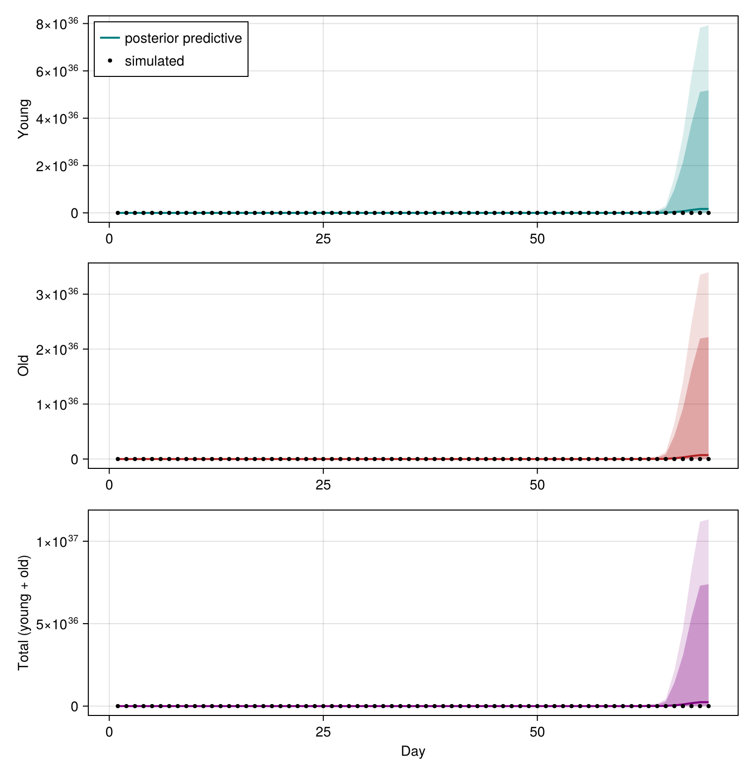
Despite the slower mixing, the 95% band covers the simulated counts on almost every day for all three streams, so the many-to-one map is recovered. A single shared young and old need no independent signal of their own, and total still lands on its simulated series because W ties it to the same shared path.
Here the single renewal process supplied one infection stratum, broadcast through W. When the strata are genuinely separate infection processes, several distinct regions each with its own latent, swap the single infection model for CombineInfections. It draws each process independently and stacks the results into the same infection-strata × time matrix Split/StrataMap already expect, so IDModel(CombineInfections([...]), Split(template, W)) maps several distinct infection processes onto streams end-to-end. For one process carried across a strata axis instead, with partially pooled per-stratum deviations, see Stratify and Partial pooling across groups. It also composes with Renewal's mixing slot, see Coupled patch models.
References
- K. Sherratt, S. Abbott, S. R. Meakin, J. Hellewell, J. D. Munday, N. Bosse, M. Jit and S. Funk. Exploring surveillance data biases when estimating the reproduction number: with insights into subpopulation transmission of COVID-19 in England. Philosophical Transactions of the Royal Society B 376, 20200283 (2021).