A Gaussian-process latent process

Any latent process that implements as_turing_model(model, n) and returns a length-n path can drive an infection model. A Gaussian process (GP) is a prior over functions, so it lets the data pick the shape of a smoothly varying quantity such as subject only to the smoothness the kernel implies. Reach for one when the roughness of the path should be learned rather than fixed in advance. AR and RandomWalk are cheaper and usually enough for local smoothing.

The package ships two GP latent models built on the same KernelFunctions.jl kernels.

• ExactGP forms the full   covariance and factorises it. Accurate, but per log-density evaluation, so use it on short series and as the accuracy reference.

• HilbertSpaceGP is the basis-function approximation of Riutort-Mayol et al. [8], building on [10]. A fixed basis makes each evaluation an   matrix–vector product, so use it for anything longer.

Two GP latent models

Both are latent models in their own right, so giving one a series length returns a length-n draw like any other component.

using ComposableTuringIDModels, Distributions, Random
Random.seed!(202)

hsgp = HilbertSpaceGP(m = 20, c = 1.5)
exact = ExactGP()
(hsgp = length(as_turing_model(hsgp, 60)()),
    exact = length(as_turing_model(exact, 60)()))

(hsgp = 60, exact = 60)

Both sample a length scale and a marginal standard deviation . HilbertSpaceGP then draws standard-normal basis weights , and ExactGP draws weights that it pushes through the Cholesky factor of the full covariance. Both are non-centred parameterisations, which NUTS handles well.

The basis depends only on n, m and c, so as_turing_model builds it before returning the model and only the matrix–vector product is differentiated. The exact GP rebuilds and differentiates its covariance and Cholesky factor on every evaluation, which is where the timing gap below comes from.

Kernels and a check against AbstractGPs

A kernel enters ExactGP through its Gram matrix and HilbertSpaceGP only through its spectral density, so either model takes SqExponentialKernel (the default), Matern32Kernel or Matern52Kernel, in order from smoothest paths to roughest.

Both models are linear in a vector of standard-normal weights, so unit vectors at fixed hyperparameters trace out that map and the Gram matrix of the result is the model's implied prior covariance. The check below compares it against the same kernel in AbstractGPs.jl.

using LinearAlgebra
using AbstractGPs: GP, cov as gp_cov
using KernelFunctions: with_lengthscale
using Turing: fix

n0, σ0, ℓ0 = 40, 1.0, 0.3          # ℓ0 is the median of the default prior
unit(k, j) = [i == j ? 1.0 : 0.0 for i in 1:k]
gram(cols) = (M = reduce(hcat, cols); M * M')
relerr(K) = norm(K - K_ref) / norm(K_ref)

K_ref = gp_cov(GP(σ0^2 * with_lengthscale(SqExponentialKernel(), ℓ0))(
    standardised_index(n0)))
K_exact = gram([fix(as_turing_model(ExactGP(), n0),
                   (ℓ = ℓ0, σ = σ0, z = unit(n0, j)))() for j in 1:n0])
K_hsgp = gram([fix(as_turing_model(HilbertSpaceGP(m = 20), n0),
                  (ℓ = ℓ0, σ = σ0, β = unit(20, j)))() for j in 1:20])

err = (exact = relerr(K_exact), hsgp = relerr(K_hsgp))
@assert err.exact < 1e-5 && err.hsgp < 1e-3   # drift fails the build
map(e -> round(e, sigdigits = 2), err)

(exact = 4.1e-7, hsgp = 0.00019)

The exact GP matches to the jitter it adds for a stable Cholesky factor, and the basis to two parts in ten thousand.

That accuracy is not uniform in , and the two knobs fail at opposite ends. The basis cannot resolve wiggles finer than , so a short length scale needs a larger m. A long one instead feels the   boundary and needs a wider c, which more basis functions will not fix.

function hsgp_relerr(ℓ, m)
    K_true = gp_cov(GP(σ0^2 * with_lengthscale(SqExponentialKernel(), ℓ))(
        standardised_index(n0)))
    K = gram([fix(as_turing_model(HilbertSpaceGP(m = m), n0),
                 (ℓ = ℓ, σ = σ0, β = unit(m, j)))() for j in 1:m])
    return norm(K - K_true) / norm(K_true)
end

ℓs = [0.1, 0.2, 0.4, 0.8]
e20, e60 = hsgp_relerr.(ℓs, 20), hsgp_relerr.(ℓs, 60)
@assert e60[1] < e20[1] / 100 && e60[4] ≈ e20[4]  # m fixes short ℓ, not long
(ℓ = ℓs, m20 = round.(e20, sigdigits = 2), m60 = round.(e60, sigdigits = 2))

(ℓ = [0.1, 0.2, 0.4, 0.8], m20 = [0.25, 0.015, 1.6e-5, 0.017], m60 = [0.00027, 7.2e-14, 1.6e-5, 0.017])

The default prior puts about a third of its mass below 0.2, so a fit that settles on a short length scale wants a larger m than the default 20. Raising m does nothing at  , where the boundary factor c sets the floor.

Simulate from an exact GP

Handing a GP to a Renewal as its rt process makes it the reproduction number. The generation interval is a serial interval discretised by Renewal, and reported cases are overdispersed counts from NegativeBinomialError.

Passing missing observations makes the composed model a prior simulator, fix pins the GP hyperparameters to a known length scale, and one seeded draw gives the data. The returned quantities include the reported cases generated_y_t and the GP path Z_t, which is . Seeding at around fifty infections keeps the early counts informative about ; from a handful, both fits would sit on the prior for the first fortnight and the comparison would measure the seed size.

si = Gamma(6.5, 0.62)
obs = NegativeBinomialError(cluster_factor = HalfNormal(0.1))
n = 70

id_model(latent) = IDModel(Renewal(; generation_time = si, rt = latent,
        initialisation = Normal(log(50), 0.1)), obs)

Random.seed!(10)
sim = fix(as_turing_model(id_model(ExactGP()), fill(missing, n), n),
    (ℓ = 0.55, σ = 0.55))()
y_obs = sim.generated_y_t
Z_true = sim.Z_t
(total_cases = sum(y_obs), peak = maximum(y_obs),
    Rt_range = round.(extrema(exp.(Z_true)), digits = 2))

(total_cases = 201221, peak = 11784, Rt_range = (0.6, 2.08))

The simulated starts near two, dips, peaks again around day 40 and falls through one near day 50, so the epidemic grows, turns over and declines.

using CairoMakie

fig_sim = Figure(; size = (760, 480))
ax_rt = Axis(fig_sim[1, 1]; ylabel = "Reproduction number Rₜ")
lines!(ax_rt, 1:n, exp.(Z_true); color = :black, linewidth = 2,
    label = "simulated truth")
hlines!(ax_rt, [1.0]; color = :grey, linestyle = :dash)
axislegend(ax_rt; position = :rt)
ax_y = Axis(fig_sim[2, 1]; xlabel = "Day", ylabel = "Reported cases")
scatter!(ax_y, 1:n, y_obs; color = :black, markersize = 7,
    label = "simulated observations")
axislegend(ax_y; position = :lt)
fig_sim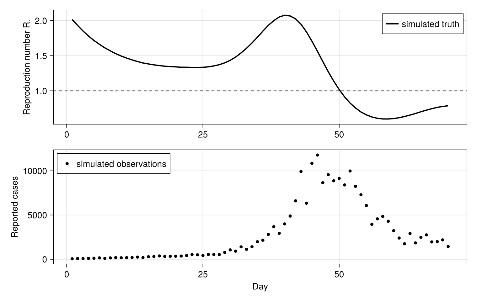

Fit both GPs and compare

Conditioning on the counts and sampling with NUTS recovers the posterior, differentiated with Mooncake, the recommended backend for this package. The helper below fits a chosen GP latent to the first n_fit days, times the run, recovers the per-draw with generated_observables and scores the posterior mean against the truth.

using Turing, Mooncake, Statistics
using ADTypes: AutoMooncake

function fit_gp(latent, n_fit)
    model = id_model(latent)
    y = y_obs[1:n_fit]
    posterior = as_turing_model(model, y, n_fit)
    time = @elapsed chain = sample(posterior,
        NUTS(0.9; adtype = AutoMooncake(; config = nothing)), 300;
        initial_params = InitFromPrior(), progress = false)
    gen = vec(generated_observables(posterior, y, chain).generated)
    Z = reduce(hcat, (g.Z_t for g in gen))          # time × draw
    Z_mean = vec(mean(Z; dims = 2))
    Z_ref = Z_true[1:n_fit]
    (; model, chain, n = n_fit, Z, Z_mean, time, cor = cor(Z_mean, Z_ref),
        rmse = sqrt(mean((Z_mean .- Z_ref) .^ 2)))
end

Random.seed!(1)
n_ex = 60
hs = fit_gp(HilbertSpaceGP(m = 20), n)
Random.seed!(1)
ex = fit_gp(ExactGP(), n_ex)

score(f) = (days = f.n, cor = round(f.cor, digits = 2),
    rmse = round(f.rmse, digits = 3), seconds = round(f.time, digits = 1))
scores() = "$(score(hs)), $(score(ex))"

@assert hs.cor>0.9 && ex.cor>0.85 "posterior mean lost the latent: $(scores())"
@assert hs.rmse<0.15 && ex.rmse<0.2 "posterior mean off the truth: $(scores())"
(hsgp = score(hs), exact = score(ex))

(hsgp = (days = 70, cor = 0.99, rmse = 0.045, seconds = 122.1), exact = (days = 60, cor = 0.99, rmse = 0.047, seconds = 386.6))

Both posterior means correlate with the simulated above 0.9 over the days they cover, and the figure below shows the two fits agreeing where they overlap. The exact GP is fit to n_ex days rather than all n because its factorisation at the full length would dominate the cost of building this page.

Those wall-clock times are single un-warmed runs over different series lengths, so read them as indicative. One gradient of each composed log-density over the same n_ex days is the like-for-like comparison, and it is what the sampler pays per leapfrog step.

using Chairmarks: @b
using DynamicPPL: LogDensityFunction, VarInfo
using LogDensityProblems: logdensity_and_gradient

composed(latent, n_fit) = as_turing_model(
    id_model(latent), y_obs[1:n_fit], n_fit)

function gradient_time(model)
    ldf = LogDensityFunction(model; adtype = AutoMooncake(; config = nothing))
    θ = VarInfo(model)[:]
    return (@b logdensity_and_gradient(ldf, θ)).time
end

grad = (hsgp = gradient_time(composed(HilbertSpaceGP(m = 20), n_ex)),
    exact = gradient_time(composed(ExactGP(), n_ex)))
round(grad.exact / grad.hsgp; sigdigits = 2)

2.7

The exact GP costs more per gradient even on the shorter series, and the gap widens with series length, which is why the approximation exists.

Posterior trajectories

  comes from the returned Z_t draws. The reported counts are scored element-wise, so their posterior predictive distribution comes from predict on the same model with the observations set to missing, stacking the y_t[i] draws into a time × draws matrix.

CI_QS = [0.025, 0.25, 0.5, 0.75, 0.975]

# time × 5 credible bands from a time × draws matrix
credible_bands(mat; qs = CI_QS) = reduce(hcat,
    (map(row -> quantile(row, q), eachrow(mat)) for q in qs))

# median line with 50% and 95% ribbons
function ci_ribbon!(ax, ts, b; color, label)
    band!(ax, ts, b[:, 1], b[:, 5]; color = (color, 0.15))
    band!(ax, ts, b[:, 2], b[:, 4]; color = (color, 0.3))
    lines!(ax, ts, b[:, 3]; color = color, linewidth = 2, label = label)
end

ts = 1:n
fig = Figure(; size = (760, 620))
ax1 = Axis(fig[1, 1]; ylabel = "Reproduction number Rₜ")
for (fit, color, label) in ((hs, :teal, "HSGP"),
    (ex, :purple, "exact (first $(n_ex) days)"))
    ci_ribbon!(ax1, 1:(fit.n), credible_bands(exp.(fit.Z)); color = color,
        label = label)
end
lines!(ax1, ts, exp.(Z_true); color = :black, linewidth = 2,
    linestyle = :dash, label = "truth")
hlines!(ax1, [1.0]; color = :grey, linestyle = :dash)
axislegend(ax1; position = :rt)

ax2 = Axis(fig[2, 1]; xlabel = "Day", ylabel = "Reported cases")
pred = predict(as_turing_model(hs.model, fill(missing, n), n), hs.chain)
yt = reduce(vcat, (permutedims(vec(pred[@varname(y_t[i])])) for i in ts))
ci_ribbon!(ax2, ts, credible_bands(yt); color = :teal,
    label = "HSGP posterior predictive")
scatter!(ax2, ts, y_obs; color = :black, markersize = 7, label = "observed")
axislegend(ax2; position = :lt)
fig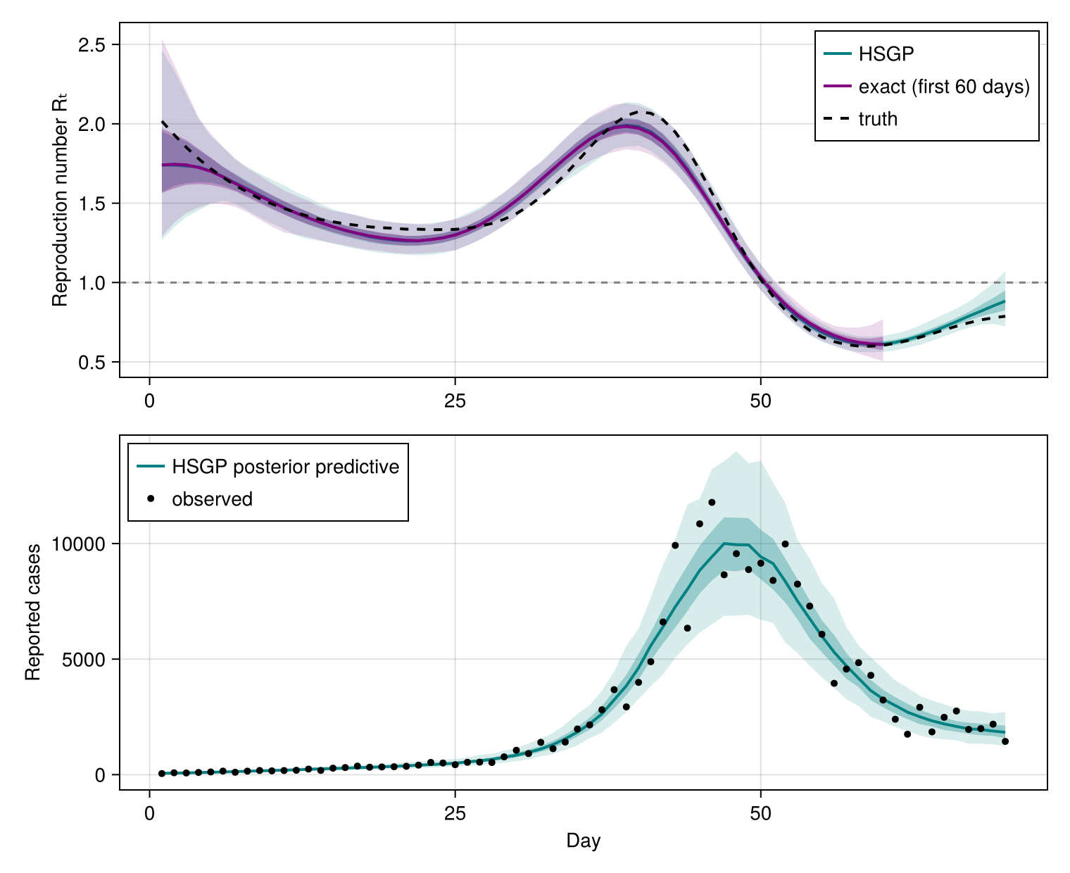

Illustrative run

This example uses a short sampler run and simulated data to stay fast to build. For a real analysis you would use more iterations, check convergence diagnostics, tune the number of basis functions m to the expected smoothness, and supply observed data.

References

2. G. Riutort-Mayol, P.-C. Bürkner, M. R. Andersen, A. Solin and A. Vehtari. Practical Hilbert space approximate Bayesian Gaussian processes for probabilistic programming. Statistics and Computing 33, 17 (2023).

3. A. Solin and S. Särkkä. Hilbert space methods for reduced-rank Gaussian process regression. Statistics and Computing 30, 419–446 (2020).