Coupled patch models

A spatial or age-stratified epidemic runs several patches over one time axis. This page builds one coupled patch model a layer at a time. Each layer is simulated and plotted before the next is added, so what the layer does is visible rather than asserted. The finished model is then fitted to data simulated from itself, to see whether the coupling is recoverable. The last two sections swap the coupling for the other options in the package, and write a new one.

Partial pooling across groups has its own tutorial and is used here without deriving it again. So does observing several streams, including the weight matrix that maps many infection strata onto fewer reported streams.

using ComposableTuringIDModels, Distributions, Random, Statistics
using CairoMakie
Random.seed!(2026)

n_strata, n_time = 3, 30
days = 1:n_time
gen_int = [0.2, 0.3, 0.3, 0.2]
patch_colours = [:steelblue, :darkorange, :seagreen]

# One innovation prior, reused by every stage, so the stages differ only in the
# layer being added.
walk = RandomWalk(init = Normal(log(1.15), 0.05),
    ϵ_t = HierarchicalNormal(std = HalfNormal(0.03)))

One figure helper serves every stage, one line per patch on shared axes.

function patch_lines(mat; ylabel, title)
    fig = Figure(; size = (720, 300))
    ax = Axis(fig[1, 1]; xlabel = "Day", ylabel = ylabel, title = title)
    for g in 1:n_strata
        lines!(ax, days, mat[g, :]; color = patch_colours[g], linewidth = 2,
            label = "Patch $g")
    end
    axislegend(ax; position = :lt)
    fig
end

Independent patches

Replicate draws one latent process per patch and stacks them into the strata × time matrix a renewal process needs.

Random.seed!(11)
independent = Renewal(gen_int; rt = Replicate(walk),
    initialisation = Normal(log(50.0), 0.2))
sim_ind = as_turing_model(independent, (n_strata, n_time))()
patch_lines(exp.(sim_ind.Z_t); ylabel = "Rₜ",
    title = "Independent patches: three unrelated paths")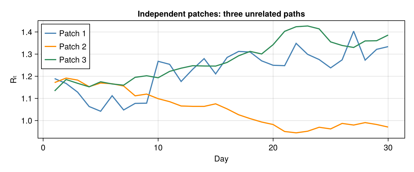

The three paths wander apart because nothing ties them together. There is no common driver and no infection pressure moving between patches.

A shared process across patches

Stratify draws the process once over time and a deviation once over the patch axis, then combines them. A Hierarchy in the across slot shrinks each patch's deviation toward the shared level.

using Accessors
Random.seed!(11)
rt_process = Stratify(walk,
    Hierarchy(; mean = Normal(0.0, 0.1), across = IID(Normal(0.0, 0.2))))
pooled = @set independent.rt = rt_process
sim_pooled = as_turing_model(pooled, (n_strata, n_time))()
patch_lines(exp.(sim_pooled.Z_t); ylabel = "Rₜ",
    title = "Shared process: one shape, three levels")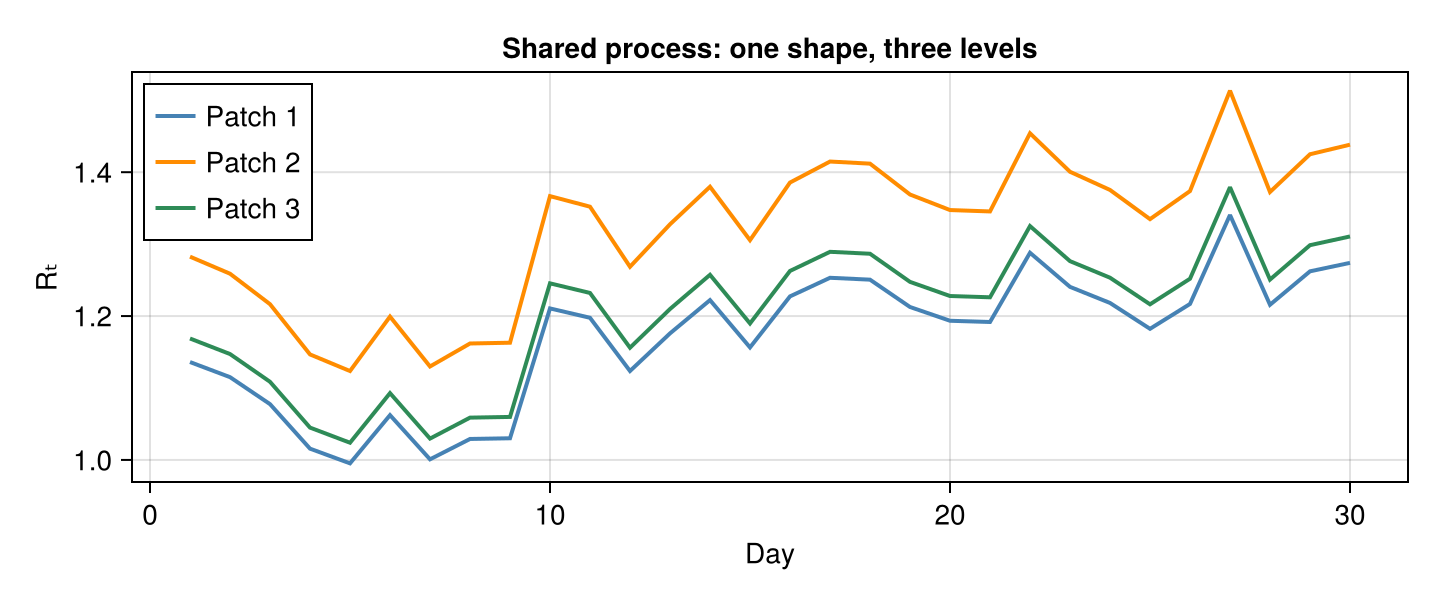

The three paths now move together and differ by a per-patch offset. Swap across for IID to pool nothing, or FixedIntercept(0.0) to collapse the patches onto one identical path.

Coupling the patches

A shared R_t is still not coupling. Each patch's incidence so far depends only on its own history. Renewal's mixing slot changes that. Every step convolves each patch's own incidence history with the generation interval, and K then redistributes the resulting pressures across patches.

K[g, h] is the force patch h puts on patch g. The diagonal is a patch's own weight. The default K = I is the uncoupled case above.

The matrix below is deliberately one-directional. Patch 1 pushes hard on patch 3 and lightly on patch 2, and nothing pushes back.

K = [1.0 0.0 0.0
     0.1 1.0 0.0
     0.4 0.0 1.0]

Random.seed!(11)
coupled = @set pooled.mixing = K
sim_coupled = as_turing_model(coupled, (n_strata, n_time))()

The seed is the same as the uncoupled run, so the R_t paths and the initial incidence are identical and every difference in incidence is the coupling.

fig = Figure(; size = (720, 320))
ax = Axis(fig[1, 1]; xlabel = "Day", ylabel = "Iₜ coupled / Iₜ uncoupled",
    title = "What the mixing matrix does to incidence")
for g in 1:n_strata
    lines!(ax, days, sim_coupled.I_t[g, :] ./ sim_pooled.I_t[g, :];
        color = patch_colours[g], linewidth = 2, label = "Patch $g")
end
hlines!(ax, [1.0]; color = :grey, linestyle = :dash)
axislegend(ax; position = :lt)
fig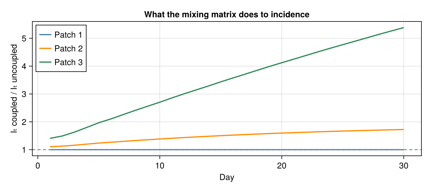

Patch 1 sits on the line because it receives nothing. Patch 3 lifts furthest and patch 2 a little, in proportion to the column of K that feeds them, and the gap widens over time because imported infections then transmit onward.

Observing the patches

Split observes each row of the infection matrix as its own stream. One error model given without stream names is used for every patch, and each stream's parameters are namespaced by stream.

Random.seed!(11)
patches = IDModel(
    coupled, Split(NegativeBinomialError(cluster_factor = HalfNormal(0.1))))

Ymiss = Matrix{Union{Missing, Float64}}(missing, n_strata, n_time)
sim = as_turing_model(patches, Ymiss)()
Rt_true = exp.(sim.Z_t)
Ydata = Float64.(reduce(vcat,
    [permutedims(sim.generated_y_t[Symbol(:group, g)]) for g in 1:n_strata]))

fig_obs = Figure(; size = (720, 320))
ax_obs = Axis(fig_obs[1, 1]; xlabel = "Day", ylabel = "Reported count",
    title = "Simulated counts (dots) around their expectation (lines)")
for g in 1:n_strata
    lines!(ax_obs, days, sim.expected_y_t[Symbol(:group, g)];
        color = patch_colours[g], linewidth = 2, label = "Patch $g")
    scatter!(ax_obs, days, Ydata[g, :]; color = patch_colours[g],
        markersize = 7)
end
axislegend(ax_obs; position = :lt)
fig_obs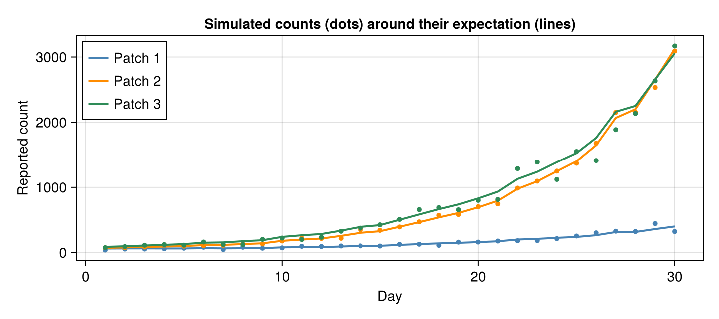

Fitting it

Everything above ran forward. Fitting the same model to the counts it produced asks what the forward runs cannot. Is a coupled, partially pooled patch process identifiable from data? We draw two chains in parallel with MCMCThreads() and differentiate with Mooncake, the recommended backend for this package (see Automatic differentiation backend).

using Turing, Mooncake
using Turing: returned
using ADTypes: AutoMooncake

posterior = as_turing_model(patches, Ydata)
chain = sample(
    posterior, NUTS(0.85; adtype = AutoMooncake(; config = nothing)),
    MCMCThreads(), 300, 2; progress = false)

┌ Info: Found initial step size
└   ϵ = 0.003125
┌ Info: Found initial step size
└   ϵ = 0.0125
┌ Warning: There were 3 divergent transitions. Consider reparameterising your model or using a smaller step size. For adaptive samplers such as NUTS and HMCDA, consider increasing `target_accept`.
└ @ Turing.Inference ~/.julia/packages/Turing/4sXd9/src/mcmc/hmc.jl:483
┌ Warning: There were 3 divergent transitions. Consider reparameterising your model or using a smaller step size. For adaptive samplers such as NUTS and HMCDA, consider increasing `target_accept`.
└ @ Turing.Inference ~/.julia/packages/Turing/4sXd9/src/mcmc/hmc.jl:483
┌ Warning: There were 6 divergent transitions. Consider reparameterising your model or using a smaller step size. For adaptive samplers such as NUTS and HMCDA, consider increasing `target_accept`.
└ @ Turing.Inference ~/.julia/packages/Turing/4sXd9/src/mcmc/hmc.jl:483

Z_t is a generated quantity, so the fitted R_t path is read back per draw and turned into credible bands.

draws = vec(returned(posterior, chain))
Rt_stack = cat((exp.(d.Z_t) for d in draws)...; dims = 3)

credible_bands(mat; qs = [0.1, 0.5, 0.9]) = reduce(hcat,
    (map(row -> quantile(row, q), eachrow(mat)) for q in qs))

patch_bands = [credible_bands(Rt_stack[g, :, :]) for g in 1:n_strata]
band_matrix(k) = permutedims(reduce(hcat, (b[:, k] for b in patch_bands)))
Rt_lo, Rt_med, Rt_hi = band_matrix(1), band_matrix(2), band_matrix(3)

fig_fit = Figure(; size = (760, 640))
for g in 1:n_strata
    ax_fit = Axis(fig_fit[g, 1]; ylabel = "Patch $g  Rₜ",
        xlabel = g == n_strata ? "Day" : "")
    band!(ax_fit, days, Rt_lo[g, :], Rt_hi[g, :]; color = (:purple, 0.25))
    lines!(ax_fit, days, Rt_med[g, :]; color = :purple, linewidth = 2,
        label = "posterior median")
    lines!(ax_fit, days, Rt_true[g, :]; color = :black, linestyle = :dash,
        linewidth = 2, label = "simulated truth")
    hlines!(ax_fit, [1.0]; color = :grey, linestyle = :dot)
    g == 1 && axislegend(ax_fit; position = :lt)
end
fig_fit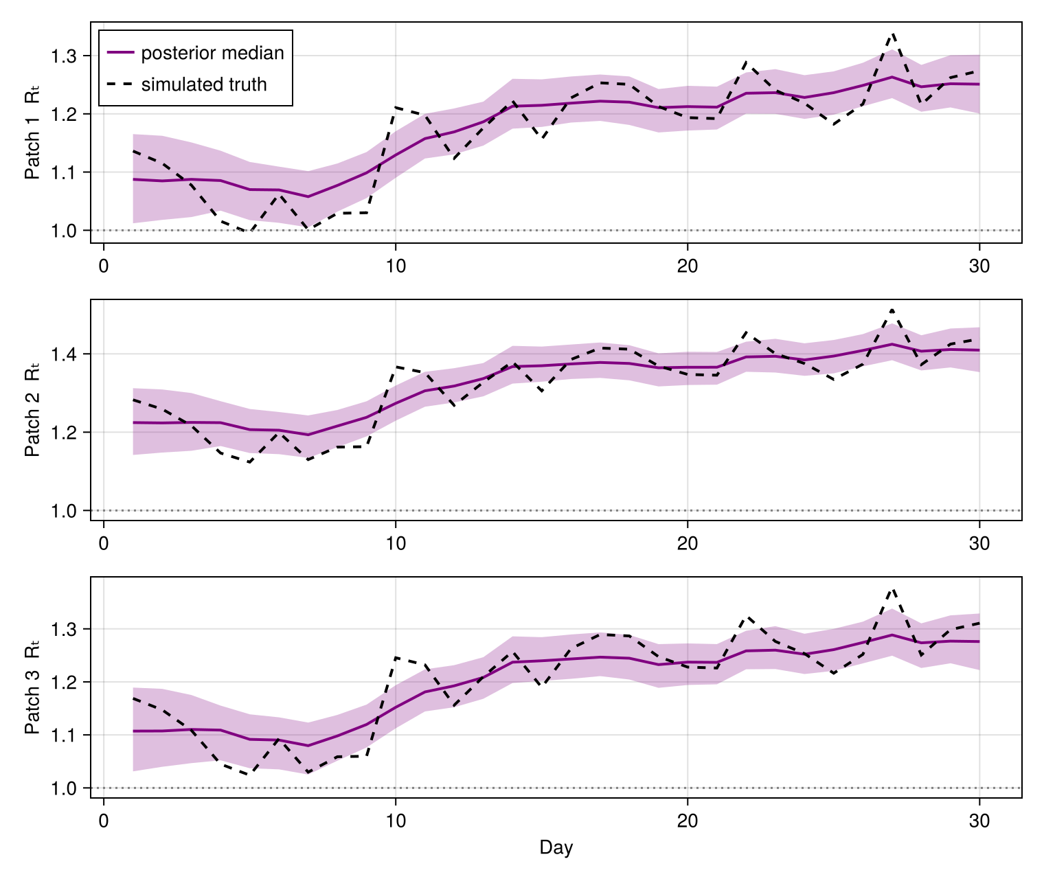

Read the dashed line against the band. Where the truth sits inside the band the process is recovered at this signal-to-noise level, and where it leaves the band it is not.

Other couplings

K above was a matrix written down by hand. Gravity builds one instead from population sizes and pairwise distances, with the three exponents drawn rather than fixed. gravity is the same calculation as a function, so the shape a set of exponents implies can be seen without fitting anything.

pop = [1.0e5, 5.0e4, 2.0e5]
dist = [0.0 10.0 30.0
        10.0 0.0 25.0
        30.0 25.0 0.0]

fig_grav = Figure(; size = (760, 280))
for (i, γ) in enumerate((0.0, 0.5, 1.0))
    ax_g = Axis(fig_grav[1, i]; title = "γ = $γ", xlabel = "From patch",
        ylabel = i == 1 ? "To patch" : "", yreversed = true,
        xticks = 1:n_strata, yticks = 1:n_strata)
    hm = heatmap!(ax_g, 1:n_strata, 1:n_strata,
        permutedims(gravity(pop, dist; α = 1.0, β = 1.0, γ = γ));
        colorrange = (0, 1))
    i == 3 && Colorbar(fig_grav[1, 4], hm)
end
fig_grav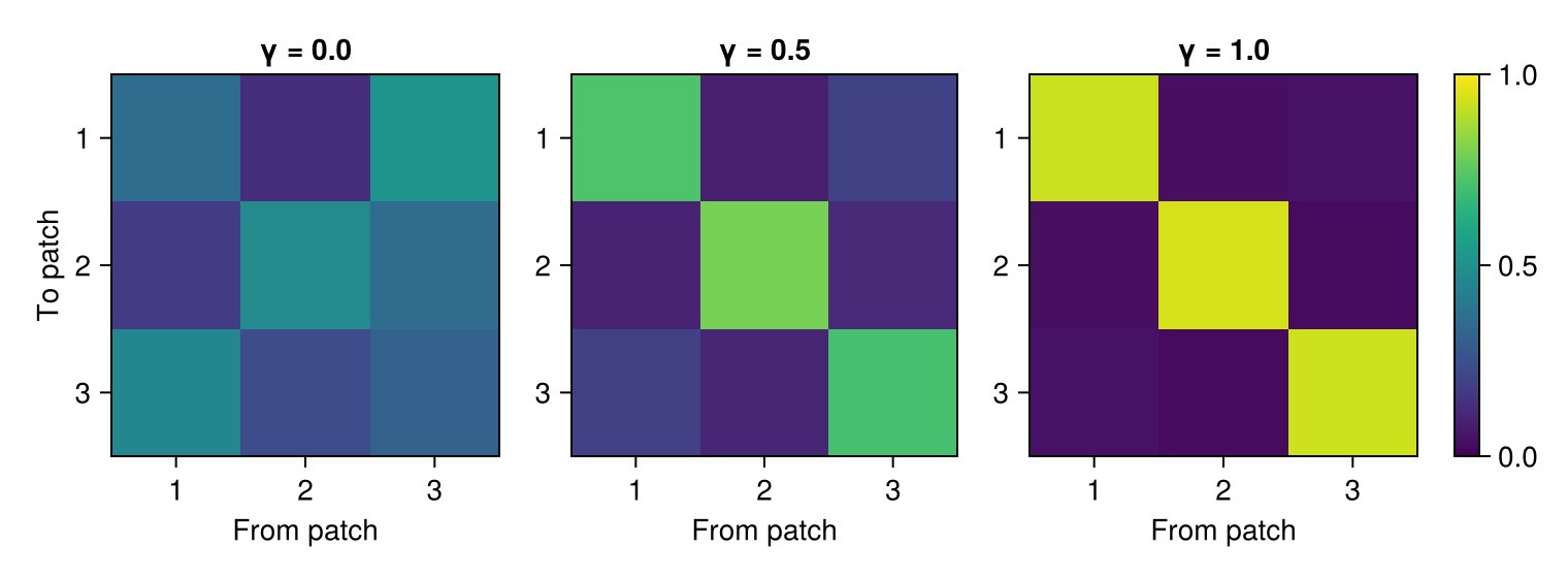

A larger distance exponent concentrates each patch's force on itself. gravity works in units of the mean population and returns rows summing to one, so K says only where a patch's force comes from and R_t carries its size. Without that split the two are confounded, since any overall scale on K does what scaling R_t does.

Handing the model rather than the matrix draws the exponents alongside everything else.

Random.seed!(11)
movement = Gravity(pop, dist; α = HalfNormal(0.5), β = HalfNormal(0.5),
    γ = HalfNormal(1.0))
gravity_model = Renewal(gen_int; rt = rt_process,
    initialisation = Normal(log(50.0), 0.2), mixing = movement)
sim_grav = as_turing_model(gravity_model, (n_strata, n_time))()
patch_lines(sim_grav.I_t; ylabel = "Iₜ",
    title = "Gravity coupling, exponents drawn from their priors")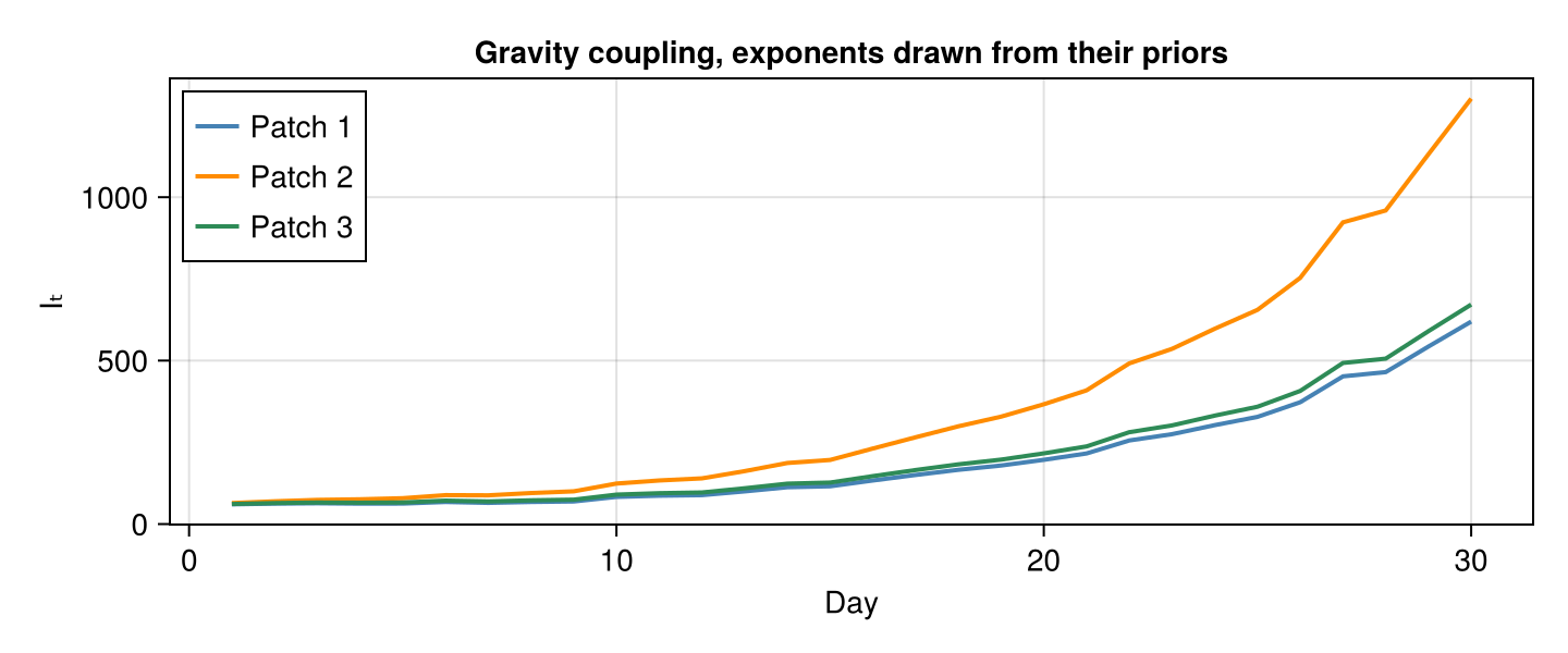

The exponents are namespaced under mixing in the chain, so a fixed and an inferred coupling differ there and nowhere else. within sets how much of a patch's force is its own, and has to be non-zero for α to be identifiable. Three patches give only three off-diagonal entries to learn from, and the two population exponents trade off against each other over that little data, so a real application needs more patches or one exponent held fixed.

Infections can also arrive from outside the modelled system altogether. ImportedCases with a stratified rate covers that. The rate is drawn before the scan, never depletes a susceptible pool, and comes from no patch's own transmission chain.

Random.seed!(11)
exogenous = Renewal(gen_int,
    ImportedCases(Stratify(FixedIntercept(-2.0), IID(Normal(0.0, 0.3))));
    rt = rt_process, initialisation = Normal(log(50.0), 0.2), mixing = K)
sim_exo = as_turing_model(exogenous, (n_strata, n_time))()
patch_lines(sim_exo.I_t ./ sim_coupled.I_t;
    ylabel = "Iₜ with / without imports",
    title = "Exogenous importation on top of the same mixing matrix")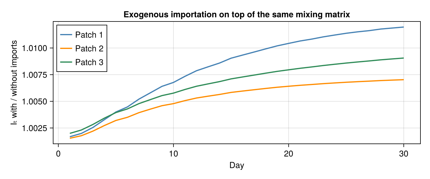

Writing a coupling

A coupling is a method of renewal_pressure taking the convolved incidence window and returning the pressure on each patch. Here the patches sit on a ring, and each takes a share of its two neighbours.

using LinearAlgebra: I

struct Ring{T}
    weight::T
end

function ComposableTuringIDModels.renewal_pressure(
        m::Ring, g, window::AbstractMatrix
    )
    own = renewal_pressure(I, g, window)
    return own .+ m.weight .* (circshift(own, 1) .+ circshift(own, -1))
end

It is passed exactly where the matrix and the Gravity model were.

Random.seed!(11)
ring = Renewal(gen_int; rt = rt_process,
    initialisation = Normal(log(50.0), 0.2), mixing = Ring(0.05))
sim_ring = as_turing_model(ring, (n_strata, n_time))()
patch_lines(sim_ring.I_t ./ sim_pooled.I_t;
    ylabel = "Iₜ ring / Iₜ uncoupled",
    title = "A coupling written from one method")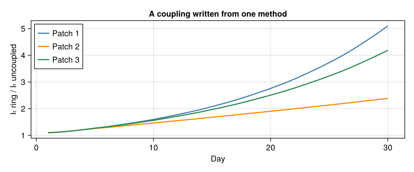

Every patch lifts, because on a ring every patch has two neighbours, and the lift compounds because imported infections then transmit onward. The process, the seeding, the observation model and the renewal recursion are all unchanged.