Declarative compartmental models with Catalyst

The SIR tutorial builds its dynamics from a hand-written vector field, and the package hand-writes that model's Jacobian too so the stiff/auto solver stays fast and stable. A hand-written Jacobian has to be re-derived, and kept in sync, for every new compartmental model.

Catalyst.jl [7] removes that step. You declare a reaction network, and Catalyst together with ModelingToolkit.jl generate the ODE system and a symbolic Jacobian for you, kept consistent by construction.

The extension's CatalystODEParams is model-agnostic. It takes any Catalyst ReactionSystem, reads off its species and rate parameters symbolically, and asks only for a prior per species and per rate. The same type builds an SIR model, an SEIR model, or a network with a vaccinated class or a second strain. Only the reactions change. This page fits the SIR network to a real outbreak, then swaps in SEIR without touching the rest of the model to show the API is generic.

Optional extension

The Catalyst path lives in an optional package extension. It loads only when you add and import Catalyst (and ModelingToolkit) alongside ComposableTuringIDModels, which keeps the heavy symbolic stack out of the default install. The hand-coded SIRParams / SEIRParams remain the zero-latency default. The declarative path is opt-in for users building new or more complex compartmental models.

Declaring and inspecting a network

We declare SIR as two reactions. Each reads like the transmission diagram, a rate constant then the species that react.

Catalyst expands these into the SIR drift and generates its Jacobian symbolically, so there is no vector field or Jacobian to write or maintain.

using ComposableTuringIDModels, Catalyst, ModelingToolkit, OrdinaryDiffEq
using Distributions, Random, Turing, LogExpFunctions, ADTypes
using CSV, DataFrames
Random.seed!(1978)

sir = @reaction_network begin
    β, S + I --> 2I
    γ, I --> R
end

Catalyst reads off the species and rate parameters we then attach priors to.

(species = species(sir), parameters = parameters(sir))

(species = SymbolicUtils.BasicSymbolicImpl.var"typeof(BasicSymbolicImpl)"{SymbolicUtils.SymReal}[S(t), I(t), R(t)], parameters = SymbolicUtils.BasicSymbolicImpl.var"typeof(BasicSymbolicImpl)"{SymbolicUtils.SymReal}[β, γ])

Building the parameter component

Loading Catalyst activates the extension that backs CatalystODEParams, though the type itself is a normal, exported ComposableTuringIDModels component. We hand it the network, a solver time span, and a prior per species and per rate, as symbolic-handle ⇒ spec pairs. A spec is either a Distribution (sampled, and named after its symbol in the chain, β, γ) or a plain number (a fixed value, not sampled, here the empty recovered class R(0)). The (u0, p) sampling contract is the same as the hand-coded parameter models, so it drops straight into an ODEProcess.

We fit the classic influenza outbreak in an English boarding school [6], taking the children confined to bed each day as a proxy for the infectious compartment.

N = 763          # children in the school

datapath = joinpath(pkgdir(ComposableTuringIDModels),
    "docs", "src", "tutorials", "data", "influenza_england_1978_school.csv")
influenza = CSV.read(datapath, DataFrame)
y_obs = influenza.in_bed            # children confined to bed each day
ts = collect(1.0:length(y_obs))     # observation times (days)
n = length(y_obs)

sir_params = CatalystODEParams(sir;
    tspan = (0.0, ts[end]),
    u0_priors = [sir.S => 0.99, sir.I => Beta(2, 200), sir.R => 0.0],
    p_priors = [sir.β => LogNormal(-0.5, 0.5), sir.γ => Gamma(8, 0.03125)])

A note on species ordering

Catalyst sorts the species and parameters when it builds the problem, so the internal layout is generally not the order you wrote the network in. We never rely on that order. CatalystODEParams samples into symbolic symbol => value maps that remake places by name, and the sol2infs link indexes the solution symbolically with the network's own handle, so it pulls the infectious compartment out by identity rather than by a hard-coded position.

sir_process = ODEProcess(
    params = sir_params,
    sol2infs = sol -> sol[sir.I, :],
    solver_options = Dict(:saveat => ts))

Composing and fitting

From here nothing is Catalyst-specific. We scale the infectious proportion to expected counts with a population TransformObservationModel and a PoissonError, assemble with IDModel, and fit.

observation = TransformObservationModel(PoissonError(), x -> softplus.(N .* x))
model = IDModel(sir_process, observation)

Use forward-mode autodiff for ODE models

The rest of these docs recommend Mooncake as the default AD backend, but ODE infection models are the exception and sample under ForwardDiff today. Reverse-mode Mooncake-driven NUTS through the ODE solver is not yet supported for the hand-coded or the Catalyst model. This is a pre-existing Turing/SciMLSensitivity integration gap (tracked in issue #46) rather than anything introduced by Catalyst. We therefore pass AutoForwardDiff() to NUTS explicitly.

posterior = as_turing_model(model, y_obs, n)
chain = sample(
    posterior, NUTS(0.95; adtype = AutoForwardDiff()),
    MCMCThreads(), 250, 2; progress = false)

┌ Info: Found initial step size
└   ϵ = 0.05
┌ Info: Found initial step size
└   ϵ = 0.025

The basic reproduction number   is a deterministic function of the rates, formed per draw from the and columns.

using Statistics
β = vec(chain[@varname(β)])
γ = vec(chain[@varname(γ)])
(β = mean(β), γ = mean(γ), R0 = mean(β ./ γ))

(β = 1.8813507324131595, γ = 0.4751685588003596, R0 = 3.961833957118316)

Prior versus posterior

Sampling the same model with Prior gives prior draws over the transmission and recovery rates. Overlaying them on the posterior with PairPlots.jl shows how sharply the boarding-school outbreak identifies the mechanistic rates.

using CairoMakie, PairPlots

prior_chain = sample(posterior, Prior(), 1000; progress = false)
pp_keys = [@varname(β), @varname(γ)]
pairplot(
    PairPlots.Series(chain[pp_keys]; label = "posterior"),
    PairPlots.Series(prior_chain[pp_keys]; label = "prior"))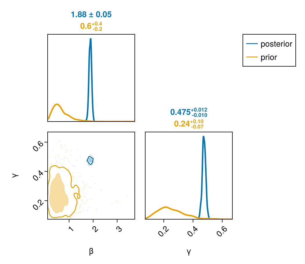

Both rates collapse from broad priors onto tight, correlated posteriors. and trade off along the   ridge that the 14 days of data constrain.

Posterior trajectories

A compartmental model has no time-varying , so the infection signal is the infectious proportion solved from the ODE. generated_observables recovers per draw, and the posterior-predictive in-bed counts come from predict on the model with the observations set to missing. Two small helpers reduce the per-draw trajectories to credible bands.

gens = vec(generated_observables(posterior, y_obs, chain).generated)
It = credible_bands(reduce(hcat, (g.I_t for g in gens)))

pred = predict(as_turing_model(model, fill(missing, n), n), chain)
yt = predictive_bands(pred, n)

fig = Figure(; size = (760, 620))
ax1 = Axis(fig[1, 1]; ylabel = "Infectious proportion I(t)")
ci_ribbon!(ax1, ts, It; color = :purple, label = "posterior median")
axislegend(ax1; position = :rt)
ax2 = Axis(fig[2, 1]; xlabel = "Day", ylabel = "Children in bed")
ci_ribbon!(ax2, ts, yt; color = :teal, label = "posterior predictive")
scatter!(ax2, ts, y_obs; color = :black, markersize = 7, label = "observed")
axislegend(ax2; position = :rt)
fig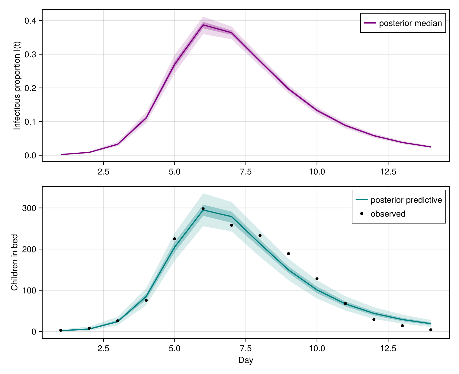

The declarative SIR dynamics, scaled by the population and Poisson observation model, reproduce the boarding-school outbreak.

The same API on a different network

The payoff of the generic path is that a different compartmental model is a different reaction network passed to the same CatalystODEParams. We add an exposed class to make SEIR, read it the same way, and fit it with no change to the observation model or the composition.

seir = @reaction_network begin
    β, S + I --> E + I
    α, E --> I
    γ, I --> R
end
(species = species(seir), parameters = parameters(seir))

(species = SymbolicUtils.BasicSymbolicImpl.var"typeof(BasicSymbolicImpl)"{SymbolicUtils.SymReal}[S(t), I(t), E(t), R(t)], parameters = SymbolicUtils.BasicSymbolicImpl.var"typeof(BasicSymbolicImpl)"{SymbolicUtils.SymReal}[β, α, γ])

The network now has four species and three rates, and Catalyst regenerates the drift and Jacobian for us. We attach a prior per species and per rate exactly as before, index the same infectious compartment symbolically, and reuse the same observation model.

seir_params = CatalystODEParams(seir;
    tspan = (0.0, ts[end]),
    u0_priors = [seir.S => 0.99, seir.E => Beta(2, 200),
        seir.I => Beta(2, 200), seir.R => 0.0],
    p_priors = [seir.β => LogNormal(-0.5, 0.4),
        seir.α => Gamma(8, 0.05), seir.γ => Gamma(8, 0.03125)])

seir_model = IDModel(
    ODEProcess(params = seir_params, sol2infs = sol -> sol[seir.I, :],
        solver_options = Dict(:saveat => ts)),
    observation)

seir_chain = sample(
    as_turing_model(seir_model, y_obs, n),
    NUTS(0.95; adtype = AutoForwardDiff()),
    MCMCThreads(), 200, 2; progress = false)
βe = vec(seir_chain[@varname(β)])
αe = vec(seir_chain[@varname(α)])
γe = vec(seir_chain[@varname(γ)])
(β = mean(βe), α = mean(αe), γ = mean(γe), R0 = mean(βe ./ γe))

(β = 3.9061366676502947, α = 1.0544922796024216, γ = 0.4877223772150541, R0 = 8.014360508798523)

Adding a fourth compartment, a vaccinated class, or a second strain is a matter of writing a different reaction network and passing it to the same type, and the vector field and Jacobian follow automatically. The Catalyst extension trades a one-off symbolic-compilation cost and a heavier dependency tree for declarative, model-agnostic dynamics.

References

2. A. Chatzilena, E. van Leeuwen, O. Ratmann, M. Baguelin and N. Demiris. Contemporary statistical inference for infectious disease models using Stan. Epidemics 29, 100367 (2019).

3. T. E. Loman, Y. Ma, V. Ilin, S. Gowda, N. Korsbo, N. Yewale, C. Rackauckas and S. A. Isaacson. Catalyst: Fast and flexible modeling of reaction networks. PLoS Computational Biology 19, e1011530 (2023).