Reporting delays and day-of-week effects
Real surveillance data is rarely a clean count of infections on the day they occur. Cases are reported after a delay, an incubation period followed by a reporting lag, and the number reported depends on the day of the week. Tools for real-time estimation such as those of Abbott et al. [3] build these features into the observation model so the latent infection signal is estimated free of reporting artefacts.
This tutorial keeps the renewal infection core of the previous example but replaces the simple observation model with a layered one. Infections are convolved through two delay distributions and then modulated by a day-of-week reporting pattern. It also shows the latent process as an ARIMA-style differenced process broadcast to a weekly timescale, and assembles everything with IDProblem. The model follows the configuration of the EpiNow2 package [3] and is fit to daily confirmed COVID-19 cases from Italy's first wave in 2020.
The model
where
A weekly latent process
The latent process is an ARIMA(2,1,1), an AR and MA combination (arma) wrapped in a DiffLatentModel to difference it once. Differencing makes the level a random walk rather than mean-reverting, which suits a reproduction number that can drift.
using ComposableTuringIDModels, Distributions, Random, Turing, Mooncake
using ADTypes: AutoMooncake
Random.seed!(20240601)

arma21 = arma(
    init = [Normal(0, 0.2), Normal(0, 0.2)],
    damp = [truncated(Normal(0.1, 0.2), 0, 1), truncated(Normal(0.1, 0.05), 0, 1)],
    θ = [truncated(Normal(0.0, 0.2), -1, 1)],
    ϵ_t = HierarchicalNormal(std = HalfNormal(0.1)))

arima211 = DiffLatentModel(; model = arma21, init = [Normal(0.3, 0.3)])
DiffLatentModel
└─ model: AR
└─ ϵ_t: MA
└─ ϵ_t: HierarchicalNormalbroadcast_weekly makes the process piecewise-constant by week, drawing a new value each week and holding it for seven days. This models
weekly_latent = broadcast_weekly(arima211)BroadcastLatentModel(RepeatBlock)
└─ model: DiffLatentModel
└─ model: AR
└─ ϵ_t: MA
└─ ϵ_t: HierarchicalNormalThe infection process
As before, a Renewal process is driven by a discretised generation interval, here a rt slot.
renewal = Renewal(; generation_time = Gamma(1.4, 1 / 0.38),
    rt = weekly_latent, initialisation = Normal(log(1.0), 1.0))
A layered observation model
We start from the NegativeBinomialError link and build outward. ascertainment_dayofweek wraps it with a partially pooled day-of-week multiplier, so reporting can be systematically higher or lower on particular weekdays.
negbin = NegativeBinomialError(cluster_factor = HalfNormal(0.1))
dayofweek_negbin = ascertainment_dayofweek(
    negbin; latent_model = HierarchicalNormal(std = HalfNormal(1.0)))
Ascertainment
├─ model: NegativeBinomialError
└─ latent: PrefixLatentModel
└─ model: BroadcastLatentModel(RepeatEach)
└─ model: TransformLatentModel
└─ model: HierarchicalNormalLatentDelay convolves the expected observations with a delay distribution discretised by double interval censoring. Two layers compose sequentially, a fixed incubation period from infection to symptom onset and then a reporting delay from onset to report whose parameters are inferred. The reporting delay is an UncertainDelay, whose LogNormal log-scale mean and standard deviation carry priors. The delay is therefore rediscretised each draw and estimated jointly with the reproduction number rather than fixed from external data.
incubation = LogNormal(1.6, 0.42)   # infection -> symptom onset (fixed)
reporting = UncertainDelay(         # symptom onset -> report (inferred)
    LogNormal, [Normal(0.58, 0.3), truncated(Normal(0.47, 0.2), 0, Inf)];
    D = 8.0)

observation = LatentDelay(LatentDelay(dayofweek_negbin, incubation), reporting)
LatentDelay
├─ model: LatentDelay
│ └─ model: Ascertainment
│ ├─ model: NegativeBinomialError
│ └─ latent: PrefixLatentModel
│ └─ model: BroadcastLatentModel(RepeatEach)
│ └─ model: TransformLatentModel
│ └─ model: HierarchicalNormal
└─ delay: UncertainDelayEach convolution shortens the expected series by length(pmf) - 1. Two stacked delays therefore need the infection process to start that many days before the first report. observation_lead_in reads the number off the assembled chain:
observation_lead_in(observation)19An IDProblem's tspan is the span of the observations, so tspan = (1, length(y)) fits every report we have. The infection process runs over the extra lead-in days to support them, derived from the chain (see What data a model needs). data_requirements says what a chain needs before it is sampled.
The data
We fit the model to the daily confirmed COVID-19 cases from Italy's first wave, the example series shipped with the EpiNow2 package and stored with the docs.
using CSV, DataFrames
datapath = joinpath(pkgdir(ComposableTuringIDModels),
    "docs", "src", "tutorials", "data", "italy_data.csv")
italy = CSV.read(datapath, DataFrame)
n = 42
y_obs = italy.confirm[1:n]
(n = n, total_cases = sum(y_obs), from = italy.date[1], to = italy.date[n])
(n = 42, total_cases = 115239, from = Dates.Date("2020-02-22"), to = Dates.Date("2020-04-03"))Assemble and fit
IDProblem ties the latent, infection, and observation models to a time span. Its as_turing_model method takes data as a named tuple with a y_t field. Passing missing values would instead simulate from the prior.
problem = IDProblem(
    infection = renewal,
    observation_model = observation,
    tspan = (1, n))
Fitting conditions on the observed reports, differentiating with the recommended Mooncake backend, described under Automatic differentiation backend. We draw two chains in parallel with MCMCThreads(), which gives a cross-chain
posterior = as_turing_model(problem, (y_t = y_obs,))
chain = sample(
    posterior, NUTS(0.95; adtype = AutoMooncake(; config = nothing)),
    MCMCThreads(), 250, 2; progress = false)
┌ Info: Found initial step size
└ ϵ = 0.000390625
┌ Info: Found initial step size
└ ϵ = 9.765625e-5DayofWeek.std is the scale of the partially pooled weekday multipliers, namespaced because the ascertainment modifier introduces a named sub-process. cluster_factor is the negative-binomial overdispersion, and delay.θ are the inferred reporting-delay parameters, the LogNormal log-mean and log-sd.
using MCMCChains
summarystats(chain)╭─FlexiSummary (9 statistics) ─────────────────────────────────────────────────╮
│ iter collapsed │
│ chain collapsed │
│ ↓ stat = [mean, std, mcse, ess_bulk, ess_tail, rhat, q5, q50, q95] │
│ │
│ Parameters (25) ── AbstractPPL.VarName │
│ Float64 init[1], diff.init[1], diff.init[2], diff.damp[1], diff.damp[2], │
│ diff.θ, diff.std, diff.ϵ_t[1], diff.ϵ_t[2], diff.ϵ_t[3], │
│ diff.ϵ_t[4], diff.ϵ_t[5], diff.ϵ_t[6], init_incidence, delay.θ[1], │
│ delay.θ[2], DayofWeek.std, DayofWeek.ϵ_t[1], DayofWeek.ϵ_t[2], │
│ DayofWeek.ϵ_t[3], DayofWeek.ϵ_t[4], DayofWeek.ϵ_t[5], │
│ DayofWeek.ϵ_t[6], DayofWeek.ϵ_t[7], cluster_factor │
│ │
│ Extras (14) │
│ Float64 n_steps, is_accept, acceptance_rate, log_density, │
│ hamiltonian_energy, hamiltonian_energy_error, │
│ max_hamiltonian_energy_error, tree_depth, numerical_error, │
│ step_size, nom_step_size, logprior, loglikelihood, logjoint │
│ │
│ Summary │
│ param mean std mcse ess_bulk ess_tail rhat … │
│ init[1] 0.7029 0.1524 0.0223 40.6132 118.3293 1.1007 … │
│ diff.init[1] 0.1101 0.1703 0.0170 98.2316 117.3275 1.0909 … │
│ diff.init[2] 0.0320 0.1239 0.0126 87.9455 72.5510 1.2213 … │
│ diff.damp[1] 0.3864 0.1933 0.1239 2.3610 14.5696 1.3617 … │
│ diff.damp[2] 0.1235 0.0416 0.0197 4.9377 81.1728 1.1588 … │
│ diff.θ 0.0965 0.1614 0.0324 25.6729 40.7123 1.0291 … │
│ diff.std 0.1461 0.0546 0.0389 1.8980 48.8754 1.5366 … │
│ diff.ϵ_t[1] -1.2391 0.5158 0.0995 32.4329 46.3388 1.1329 … │
│ diff.ϵ_t[2] -0.6113 0.5741 0.1391 20.3374 46.6014 1.0009 … │
│ diff.ϵ_t[3] -1.2382 0.7715 0.6560 1.5434 54.9111 1.7938 … │
│ diff.ϵ_t[4] -0.6225 1.1314 0.9358 1.5458 20.5884 1.7582 … │
│ diff.ϵ_t[5] -0.3051 0.6045 0.1408 21.8512 37.9187 1.0163 … │
│ diff.ϵ_t[6] 0.9012 0.9430 0.7213 1.7365 19.3498 1.6018 … │
│ init_incide… 0.1636 0.6015 0.0993 39.7147 31.9879 1.0329 … │
│ delay.θ[1] 0.5906 0.2559 0.0523 24.6016 145.3608 1.0163 … │
│ delay.θ[2] 0.5166 0.1543 0.0315 24.6515 182.2255 1.0104 … │
│ DayofWeek.s… 0.0630 0.0731 0.0533 1.4500 15.5291 1.8997 … │
│ DayofWeek.ϵ… -0.7521 0.6446 0.4489 2.1921 29.8292 1.4474 … │
│ DayofWeek.ϵ… 0.0092 0.9853 0.7963 1.5149 11.1215 1.7890 … │
│ DayofWeek.ϵ… 0.3312 0.5726 0.0848 34.8615 70.8356 1.2168 … │
│ DayofWeek.ϵ… 0.6702 0.7590 0.5526 2.4410 56.8052 1.4425 … │
│ DayofWeek.ϵ… -0.2269 1.2155 1.0384 1.4451 14.6439 1.8790 … │
│ DayofWeek.ϵ… -0.4560 0.7139 0.1432 21.5242 67.7761 1.0818 … │
│ DayofWeek.ϵ… 0.6297 0.6751 0.3245 4.7689 34.1761 1.1676 … │
│ cluster_fac… 0.2100 0.0316 0.0183 2.9449 86.8234 1.2622 … │
╰──────────────────────────────────────────────────────────────────────────────╯The day-of-week effect, the reporting delay, and the weekly reproduction number were all estimated jointly. Any of them can be swapped, fixed, or removed by editing one line of the composition above.
Prior versus posterior
Sampling the same model with Prior gives a prior draw over the same parameters. Overlaying it on the posterior with PairPlots.jl shows which parameters the six weeks of Italian data moved.
using CairoMakie, PairPlots

prior_chain = sample(posterior, Prior(), 1000; progress = false)
pp_keys = [@varname(diff.damp), @varname(diff.θ),
    @varname(diff.std), @varname(cluster_factor)]
pairplot(
    PairPlots.Series(chain[pp_keys]; label = "posterior"),
    PairPlots.Series(prior_chain[pp_keys]; label = "prior"))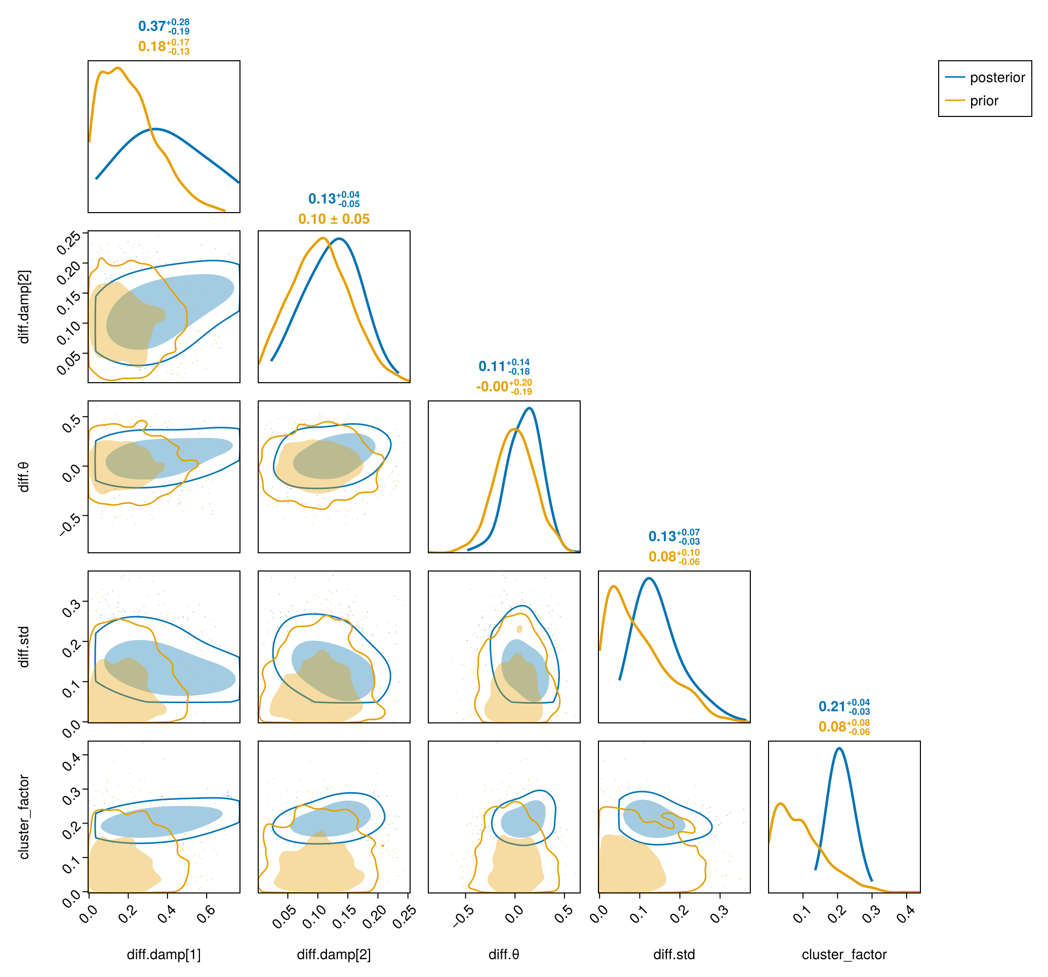
The innovation scale diff.std) and the negative-binomial overdispersion (cluster_factor) tighten under the data. The autoregressive damping (diff.damp) and moving-average (diff.θ) coefficients of the ARIMA process stay close to their weakly informative priors.
Posterior trajectories
generated_observables. The reports predict on the model with the observations set to missing. Two small helpers reduce the per-draw trajectories to credible bands.
gens = vec(generated_observables(posterior, (y_t = y_obs,), chain).generated)
Rt = credible_bands(reduce(hcat, (exp.(g.Z_t) for g in gens)))

pred = predict(as_turing_model(problem, (y_t = fill(missing, n),)), chain)
yt = predictive_bands(pred, n)

lead_in = observation_lead_in(observation)
infection_days = (1 - lead_in):n

fig = Figure(; size = (760, 620))
ax1 = Axis(fig[1, 1]; ylabel = "Reproduction number Rₜ")
ci_ribbon!(ax1, infection_days, Rt; color = :purple,
    label = "posterior median")
hlines!(ax1, [1.0]; color = :grey, linestyle = :dash)
vlines!(ax1, [0.5]; color = :grey, linestyle = :dot)
axislegend(ax1; position = :rt)
ax2 = Axis(fig[2, 1]; xlabel = "Day, numbered from the first report",
    ylabel = "Confirmed cases")
ci_ribbon!(ax2, 1:n, yt; color = :teal, label = "posterior predictive")
scatter!(ax2, 1:n, y_obs; color = :black, markersize = 7, label = "observed")
vlines!(ax2, [0.5]; color = :grey, linestyle = :dot)
axislegend(ax2; position = :lt)
linkxaxes!(ax1, ax2)
hidexdecorations!(ax1; grid = false)
fig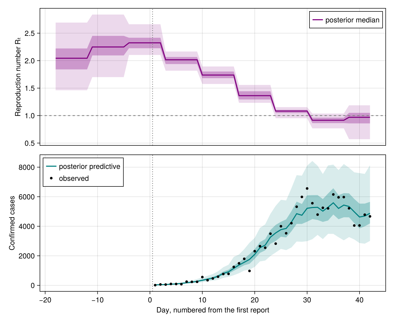
Both panels are drawn on one calendar, numbered so that day 1 is the first Italian report. The
The weekly
A time-varying reporting pattern
The day-of-week multiplier above is static, one weekly profile held fixed across the series. Reporting behaviour can itself drift as testing capacity changes or weekend effects strengthen, and the same composition expresses that. The ascertainment modifier takes any latent model, so replacing the pooled HierarchicalNormal weekday effect with a BroadcastLatentModel over a process that evolves week to week turns the fixed profile into a time-varying one, at the cost of more latent parameters. The change is again local to the observation model, leaving the infection and latent
The reporting delay can drift in the same way, through the same seam. An UncertainDelay parameter is a prior slot like any other, so replacing its constant log-mean prior with a RandomWalk makes the delay distribution itself time-varying. It is then rediscretised at each time point and applied with a per-time convolution, while the log-scale spread keeps a constant prior.
using Accessors
drifting = UncertainDelay(
    LogNormal, [RandomWalk(), truncated(Normal(0.47, 0.2), 0, Inf)]; D = 8.0)
tv_observation = @set observation.delay = drifting
LatentDelay
├─ model: LatentDelay
│ └─ model: Ascertainment
│ ├─ model: NegativeBinomialError
│ └─ latent: PrefixLatentModel
│ └─ model: BroadcastLatentModel(RepeatEach)
│ └─ model: TransformLatentModel
│ └─ model: HierarchicalNormal
└─ delay: UncertainDelay
└─ params[1]: RandomWalk
└─ ϵ_t: HierarchicalNormalAs with the weekday profile we flag rather than fit it here, because a delay that drifts day to day asks more of six weeks of data than they can answer.
References
- S. Abbott, J. Hellewell, R. N. Thompson, K. Sherratt, H. P. Gibbs, N. I. Bosse, J. D. Munday, S. Meakin, E. L. Doughty, J. Y. Chun and others. Estimating the time-varying reproduction number of SARS-CoV-2 using national and subnational case counts. Wellcome Open Research 5, 112 (2020).