An SIR compartmental model

The renewal equation is one way to generate infections, but it is not the only one. Mechanistic compartmental models describe transmission with a system of ordinary differential equations (ODEs). Chatzilena et al. [6] showed how to embed such an ODE in a Bayesian model and infer its parameters, using a classic influenza outbreak in an English boarding school as their example.

This tutorial swaps the renewal infection process for an ODEProcess built from SIRParams, keeping the same composable observation machinery. Infections come from solving the SIR equations with the SciML stack [5] rather than from a bespoke solver.

The model

, , are population proportions; is the transmission rate, the recovery rate, and the population size. The softplus link smoothly scales the infected proportion to expected counts while staying positive even if the solver returns a small negative value near zero.

The infection process

SIRParams declares priors for the transmission rate, recovery rate, and initial infected proportion, over a solver time span. We use weakly informative priors that keep the basic reproduction number   in a plausible range for influenza and bounded away from the   ( ) singularity.

using ComposableTuringIDModels, Distributions, Random, Turing, LogExpFunctions
using ADTypes: AutoForwardDiff
using CSV, DataFrames
Random.seed!(1978)

N = 763          # children in the school

datapath = joinpath(pkgdir(ComposableTuringIDModels),
    "docs", "src", "tutorials", "data", "influenza_england_1978_school.csv")
influenza = CSV.read(datapath, DataFrame)
y_obs = influenza.in_bed            # children confined to bed each day
ts = collect(1.0:length(y_obs))     # observation times (days)
n = length(y_obs)

sir_params = SIRParams(
    tspan = (0.0, ts[end]),
    infectiousness = LogNormal(-0.5, 0.5),
    recovery_rate = Gamma(8, 0.03125),
    initial_prop_infected = Beta(2, 200))

Chatzilena et al. [6] fit this to a 1978 influenza outbreak in an English boarding school, taking the number of children "in bed" each day as a proxy for the infected compartment. Of the 763 children, 512 fell ill over 14 days.

ODEProcess composes those parameters with a solver and a sol2infs link that pulls the infected compartment out of the ODE solution. This is the standard SciML pattern — a problem definition composed with a solution method — specialised to probabilistically sampled parameters. The default solver switches between explicit and implicit methods, which keeps the solve robust when the sampler proposes stiff parameter values.

# Pull the infected compartment from the ODE solution. A solve that fails under
# an extreme sampler proposal returns fewer than `n` saved points; map that to a
# series the observation likelihood rejects, so the sampler steps away rather
# than erroring on the shortened series.
function infected(sol)
    infs = sol[2, :]
    length(infs) == n ? infs : fill(eltype(infs)(Inf), n)
end

sir_process = ODEProcess(
    params = sir_params,
    sol2infs = infected,
    solver_options = Dict(:saveat => ts))

The observation model

The ODE returns the infected proportion ; we scale it to counts with the population size and a softplus transform using TransformObservationModel, then link to data with a PoissonError.

observation = TransformObservationModel(PoissonError(), x -> softplus.(N .* x))

A compartmental model needs no time-varying latent process — the dynamics are fully determined by the ODE parameters — so the ODEProcess carries no latent process at all (its Z_t generated quantity is nothing). IDModel assembles the infection and observation parts exactly as in the renewal examples.

model = IDModel(sir_process, observation)

Fit

Fitting recovers the SIR parameters from the observed "in bed" counts. This page differentiates with ForwardDiff, not the package's recommended Mooncake default: reverse-mode (Mooncake-driven) NUTS through the ODE solver is not available yet — a pre-existing Turing + Mooncake + SciMLSensitivity integration gap that affects every ODE infection model (tracked in issue #46). Forward-mode autodiff is a good fit here anyway, for a system this small. We draw two chains in parallel with MCMCThreads() so a cross-chain is available:

posterior = as_turing_model(model, y_obs, n)
chain = sample(
    posterior, NUTS(0.95; adtype = AutoForwardDiff()),
    MCMCThreads(), 250, 2; progress = false)

┌ Info: Found initial step size
└   ϵ = 0.05
┌ Info: Found initial step size
└   ϵ = 0.003125
┌ Warning: Verbosity toggle: dt_epsilon
│  Initial timestep too small (near machine epsilon), using default: dt = 1.0e-6
└ @ OrdinaryDiffEqCore ~/.julia/packages/OrdinaryDiffEqCore/NVUZl/src/initdt.jl:222

sample returns a FlexiChains chain, which summarystats summarises directly — no conversion step:

using MCMCChains
summarystats(chain)

╭─FlexiSummary (9 statistics) ─────────────────────────────────────────────────╮
│   iter    collapsed                                                          │
│   chain   collapsed                                                          │
│ ↓ stat  = [mean, std, mcse, ess_bulk, ess_tail, rhat, q5, q50, q95]          │
│                                                                              │
│ Parameters (3) ── AbstractPPL.VarName                                        │
│  Float64  β, γ, I₀                                                           │
│                                                                              │
│ Extras (14)                                                                  │
│  Float64  n_steps, is_accept, acceptance_rate, log_density,                  │
│           hamiltonian_energy, hamiltonian_energy_error,                      │
│           max_hamiltonian_energy_error, tree_depth, numerical_error,         │
│           step_size, nom_step_size, logprior, loglikelihood, logjoint        │
│                                                                              │
│ Summary                                                                      │
│   param    mean     std    mcse  ess_bulk  ess_tail    rhat      q5  …       │
│       β  1.8657  0.0537  0.0091   35.7174   81.2519  1.0304  1.7759  …       │
│       γ  0.4778  0.0110  0.0006  354.8759  314.8640  1.0033  0.4606  …       │
│      I₀  0.0006  0.0001  0.0000   36.3594   69.3423  1.0246  0.0004  …       │
╰──────────────────────────────────────────────────────────────────────────────╯

The posterior gives the transmission and recovery rates directly, and the basic reproduction number   is a deterministic function of them. Individual parameter draws are read by name with vec(chain[@varname(...)]), from which the derived is formed per draw:

using Turing: @varname
using Statistics
β = vec(chain[@varname(β)])
γ = vec(chain[@varname(γ)])
R0 = β ./ γ
(β = mean(β), γ = mean(γ), R0 = mean(R0))

(β = 1.8656651290090684, γ = 0.47779780127673344, R0 = 3.9067004019434144)

Prior versus posterior

Sampling the same model with Prior gives a prior draw over the transmission rate , recovery rate and initial infected proportion . Overlaying it on the posterior with PairPlots.jl shows how sharply the boarding-school outbreak identifies the mechanistic parameters.

using CairoMakie, PairPlots

prior_chain = sample(posterior, Prior(), 1000; progress = false)
pp_keys = [@varname(β), @varname(γ), @varname(I₀)]
pairplot(
    PairPlots.Series(chain[pp_keys]; label = "posterior"),
    PairPlots.Series(prior_chain[pp_keys]; label = "prior"))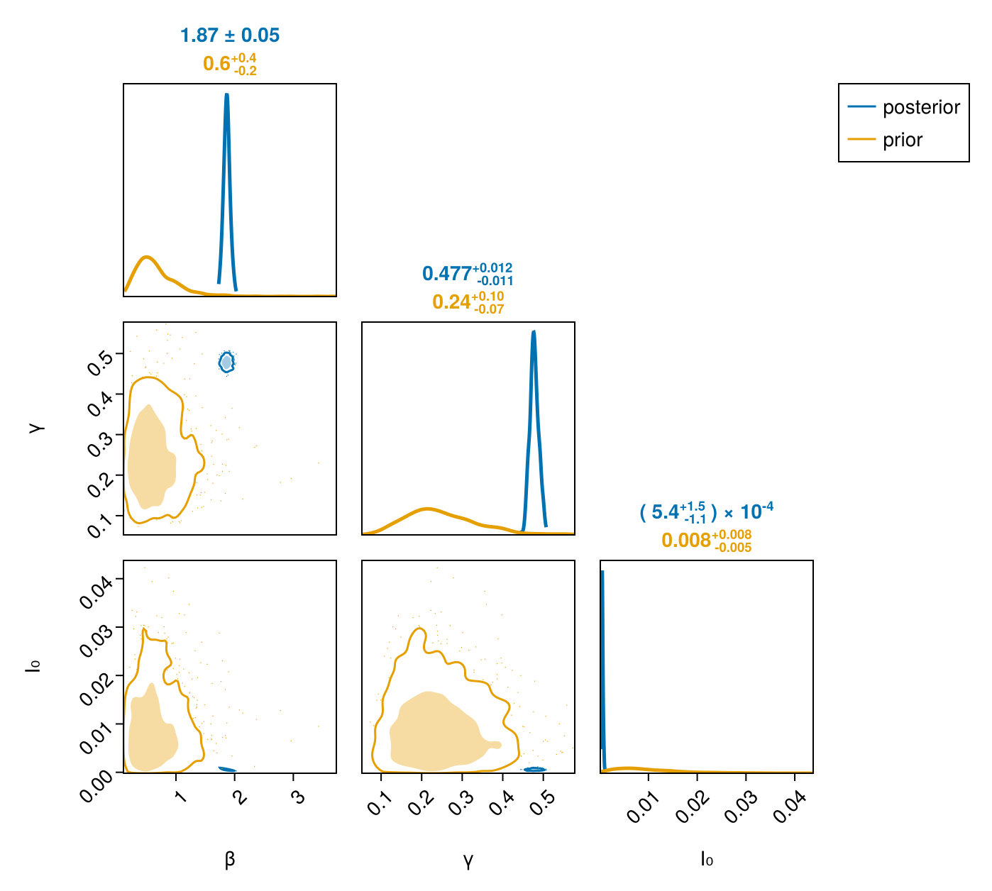

All three parameters collapse from broad priors onto tight, correlated posteriors — and trade off along the   ridge that the 14 days of data constrain.

Posterior trajectories

A compartmental model has no time-varying (its generated quantity is nothing); the infection signal is the infectious proportion solved from the ODE. generated_observables recovers per draw, and the posterior-predictive in-bed counts come from predict on the model with the observations set to missing. Two small helpers reduce the per-draw trajectories to credible bands.

gens = vec(generated_observables(posterior, y_obs, chain).generated)
It = credible_bands(reduce(hcat, (g.I_t for g in gens)))

pred = predict(as_turing_model(model, fill(missing, n), n), chain)
yt = predictive_bands(pred, n)

fig = Figure(; size = (760, 620))
ax1 = Axis(fig[1, 1]; ylabel = "Infectious proportion I(t)")
ci_ribbon!(ax1, ts, It; color = :purple, label = "posterior median")
axislegend(ax1; position = :rt)
ax2 = Axis(fig[2, 1]; xlabel = "Day", ylabel = "Children in bed")
ci_ribbon!(ax2, ts, yt; color = :teal, label = "posterior predictive")
scatter!(ax2, ts, y_obs; color = :black, markersize = 7, label = "observed")
axislegend(ax2; position = :rt)
fig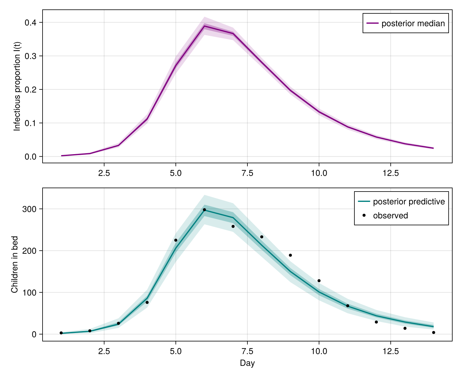

The mechanistic infectious-proportion curve peaks mid-outbreak, and the posterior-predictive in-bed counts bracket the observed epidemic curve — the SIR dynamics, scaled by the population and Poisson observation model, reproduce the boarding-school outbreak.

Adding a stochastic ascertainment process

The deterministic model assumes the SIR equations describe the data exactly up to Poisson counting noise. Real outbreaks rarely oblige: the compartmental model is an approximation, and reporting intensity drifts over time. Chatzilena et al. [6] therefore also consider a stochastic variant in which a latent autoregressive process on the log scale modulates the expected counts, absorbing variation the mechanistic part cannot explain:

Setting   for all recovers the deterministic model, so the two are nested. In this package the process is exactly the AR latent model already used for in the renewal examples — here it modulates the observation process rather than infections. An Ascertainment modifier wraps the Poisson link and carries that latent process; the population TransformObservationModel is re-applied on the outside. No part of the infection model changes. The priors are weakly informative: damping near zero (highly autocorrelated increments), an initial state near zero (no baseline adjustment), and a small innovation standard deviation.

ascertainment = AR(
    damp = [HalfNormal(0.005)],
    init = [Normal(0, 0.001)],
    ϵ_t = HierarchicalNormal(std = HalfNormal(0.02)))

stochastic_obs = TransformObservationModel(
    Ascertainment(model = PoissonError(), latent_model = ascertainment),
    x -> softplus.(N .* x))

stochastic_model = IDModel(sir_process, stochastic_obs)

Swapping the deterministic observation model for the stochastic one is a single structural change — the SIR infection process is reused untouched — and the composed model is fit exactly as before. The ascertainment process adds latent parameters, so we raise the NUTS target acceptance rate a little to keep the sampler stable through the ODE solve.

stochastic_chain = sample(
    as_turing_model(stochastic_model, y_obs, n),
    NUTS(0.95; adtype = AutoForwardDiff()),
    MCMCThreads(), 250, 2; progress = false)

┌ Warning: Verbosity toggle: dt_epsilon
│  Initial timestep too small (near machine epsilon), using default: dt = 1.0e-6
└ @ OrdinaryDiffEqCore ~/.julia/packages/OrdinaryDiffEqCore/NVUZl/src/initdt.jl:222
┌ Info: Found initial step size
└   ϵ = 0.00078125
┌ Warning: Verbosity toggle: dt_epsilon
│  Initial timestep too small (near machine epsilon), using default: dt = 1.0e-6
└ @ OrdinaryDiffEqCore ~/.julia/packages/OrdinaryDiffEqCore/NVUZl/src/initdt.jl:222
┌ Warning: Verbosity toggle: dt_epsilon
│  Initial timestep too small (near machine epsilon), using default: dt = 1.0e-6
└ @ OrdinaryDiffEqCore ~/.julia/packages/OrdinaryDiffEqCore/NVUZl/src/initdt.jl:222
┌ Warning: Verbosity toggle: dt_epsilon
│  Initial timestep too small (near machine epsilon), using default: dt = 1.0e-6
└ @ OrdinaryDiffEqCore ~/.julia/packages/OrdinaryDiffEqCore/NVUZl/src/initdt.jl:222
┌ Warning: Verbosity toggle: dt_epsilon
│  Initial timestep too small (near machine epsilon), using default: dt = 1.0e-6
└ @ OrdinaryDiffEqCore ~/.julia/packages/OrdinaryDiffEqCore/NVUZl/src/initdt.jl:222
┌ Warning: Verbosity toggle: dt_epsilon
│  Initial timestep too small (near machine epsilon), using default: dt = 1.0e-6
└ @ OrdinaryDiffEqCore ~/.julia/packages/OrdinaryDiffEqCore/NVUZl/src/initdt.jl:222
┌ Info: Found initial step size
└   ϵ = 0.0015625

The SIR parameters keep their flat names (β, γ, I₀); the ascertainment process contributes its own block, prefixed Ascertainment. because modifiers that introduce a named sub-process prefix their variables to keep them distinct. summarystats shows both blocks, including the ascertainment innovation scale (Ascertainment.std), which quantifies how much observation-level noise the latent process absorbed:

summarystats(stochastic_chain)

╭─FlexiSummary (9 statistics) ─────────────────────────────────────────────────╮
│   iter    collapsed                                                          │
│   chain   collapsed                                                          │
│ ↓ stat  = [mean, std, mcse, ess_bulk, ess_tail, rhat, q5, q50, q95]          │
│                                                                              │
│ Parameters (20) ── AbstractPPL.VarName                                       │
│  Float64  β, γ, I₀, Ascertainment.ar_init[1], Ascertainment.damp_AR,         │
│           Ascertainment.ρ, Ascertainment.std, Ascertainment.ϵ_t[1],          │
│           Ascertainment.ϵ_t[2], Ascertainment.ϵ_t[3], Ascertainment.ϵ_t[4],  │
│           Ascertainment.ϵ_t[5], Ascertainment.ϵ_t[6], Ascertainment.ϵ_t[7],  │
│           Ascertainment.ϵ_t[8], Ascertainment.ϵ_t[9], Ascertainment.ϵ_t[10], │
│           Ascertainment.ϵ_t[11], Ascertainment.ϵ_t[12],                      │
│           Ascertainment.ϵ_t[13]                                              │
│                                                                              │
│ Extras (14)                                                                  │
│  Float64  n_steps, is_accept, acceptance_rate, log_density,                  │
│           hamiltonian_energy, hamiltonian_energy_error,                      │
│           max_hamiltonian_energy_error, tree_depth, numerical_error,         │
│           step_size, nom_step_size, logprior, loglikelihood, logjoint        │
│                                                                              │
│ Summary                                                                      │
│          param     mean     std    mcse  ess_bulk  ess_tail    rhat  …       │
│              β   1.2624  0.6166  0.6108    1.3741   29.7965  2.1263  …       │
│              γ   1.2741  0.7900  0.7836    1.3464   21.9270  2.1263  …       │
│             I₀   0.3433  0.3431  0.3404    1.3365   38.1665  2.1263  …       │
│   Ascertainme…  -0.0220  0.0229  0.0222    1.3480   21.8876  2.1263  …       │
│   Ascertainme…   0.9886  1.0068  0.9879    1.3248   10.8746  2.1263  …       │
│   Ascertainme…   0.9886  1.0068  0.9879    1.3248   10.8746  2.1263  …       │
│   Ascertainme…   0.6101  0.5553  0.5507    1.3152   11.6514  2.1263  …       │
│   Ascertainme…   0.1777  0.7889  0.2386   11.5198   28.6046  1.9276  …       │
│   Ascertainme…  -0.1446  0.7091  0.1924   23.9245   40.5252  1.9314  …       │
│   Ascertainme…   0.1869  0.8622  0.5599    3.4831   36.2579  2.0356  …       │
│   Ascertainme…   1.0831  0.9975  0.7790    1.8674   31.4171  2.0678  …       │
│   Ascertainme…  -0.5715  0.8308  0.6862    1.6853   69.8402  2.0925  …       │
│   Ascertainme…  -0.0142  0.8012  0.6773    1.4241   34.3888  2.1263  …       │
│   Ascertainme…   0.3821  0.6768  0.3890    3.2191   16.6886  2.1228  …       │
│   Ascertainme…   1.1646  0.6488  0.1564    7.4126   16.7105  2.1178  …       │
│   Ascertainme…   0.0546  1.0256  0.9252    1.3449   23.2294  2.1263  …       │
│   Ascertainme…   0.6117  0.6222  0.1141   30.0159   37.1944  2.1046  …       │
│   Ascertainme…  -0.7835  0.6918  0.1274   30.4487   34.1724  2.0986  …       │
│   Ascertainme…  -1.3677  0.7813  0.4952    2.9171   33.2560  2.1195  …       │
│   Ascertainme…  -0.3390  0.8480  0.6121    2.2710   37.6632  2.1274  …       │
╰──────────────────────────────────────────────────────────────────────────────╯

The basic reproduction number is recovered as before — a derived quantity formed per draw from the sampled and — and the fitted ascertainment scale is small:

βs = vec(stochastic_chain[@varname(β)])
γs = vec(stochastic_chain[@varname(γ)])
asc_std = vec(stochastic_chain[@varname(Ascertainment.std)])
(R0 = mean(βs ./ γs), ascertainment_sigma = mean(asc_std))

(R0 = 2.0930291058792547, ascertainment_sigma = 0.6101371042422392)

Because the deterministic model is the   special case, the two fits are directly comparable on this real outbreak:

(deterministic_R0 = mean(R0), stochastic_R0 = mean(βs ./ γs))

(deterministic_R0 = 3.9067004019434144, stochastic_R0 = 2.0930291058792547)

The SIR model is an approximation to the real transmission dynamics, so here the stochastic ascertainment process soaks up systematic departures from the SIR mean, guarding the mechanistic against that bias — the reason Chatzilena et al. [6] introduce it.

References

2. C. Rackauckas and Q. Nie. DifferentialEquations.jl – a performant and feature-rich ecosystem for solving differential equations in Julia. Journal of Open Research Software 5 (2017).

3. A. Chatzilena, E. van Leeuwen, O. Ratmann, M. Baguelin and N. Demiris. Contemporary statistical inference for infectious disease models using Stan. Epidemics 29, 100367 (2019).