
Renewal model with negative-binomial reporting
The renewal equation expresses new infections as a function of past infections weighted by the generation interval, scaled by a time-varying reproduction number
This tutorial builds that model from two composed parts and fits it to the test-confirmed COVID-19 cases from South Korea that Mishra et al. [2] analysed. The parts are a Renewal infection process carrying an autoregressive latent process for NegativeBinomialError observation model. The latent
The model
Components
The latent process is a second-order autoregressive model on HierarchicalNormal innovation term, matching Mishra et al. [2]. Strong autocorrelation in the reproduction number is encoded by a first damping prior concentrated near one,
using ComposableTuringIDModels, Distributions, Random, Turing, Mooncake
using ADTypes: AutoMooncake
Random.seed!(1234)

latent = AR(
    damp = [truncated(Normal(0.8, 0.05), 0, 1),
        truncated(Normal(0.1, 0.05), 0, 1)],
    init = [Normal(0.0, 0.2), Normal(0.0, 0.2)],
    ϵ_t = HierarchicalNormal(std = HalfNormal(0.1)))
AR
└─ ϵ_t: HierarchicalNormalThe infection process needs a discrete generation interval. Renewal takes a continuous distribution and discretises it with double interval censoring [9], using CensoredDistributions.jl. Following Mishra et al. [2] we use a Renewal is the only infection model that carries a generation interval, because it is the only one that uses one. It couples that interval to the latent rt slot and a prior for the initial infections.
renewal = Renewal(; generation_time = Gamma(6.5, 0.62),
    rt = latent, initialisation = Normal(log(1.0), 0.1))
renewal.gen_int
8-element Vector{Float64}:
0.026663134095601098
0.14059778064943768
0.2502660305615845
0.24789569560506872
0.1731751163417783
0.09635404000022221
0.045734375752163825
0.01931382699414364The stored gen_int is a probability vector, the continuous serial interval binned into daily weights that sum to one. Double interval censoring is not the same as evaluating the continuous density at integer days. It accounts for both the primary and secondary events falling anywhere within their days [9]. The lag-0 bin is dropped and the weights renormalised over the days kept, so the discrete interval is a little shorter and a little tighter than the
using Statistics
lags = 1:length(renewal.gen_int)
discrete_mean = sum(lags .* renewal.gen_int)
discrete_sd = sqrt(sum((lags .- discrete_mean) .^ 2 .* renewal.gen_int))
serial_interval = Gamma(6.5, 0.62)
(discrete = round.((discrete_mean, discrete_sd), digits = 2),
    continuous = round.((mean(serial_interval), std(serial_interval)), digits = 2))
(discrete = (3.97, 1.53), continuous = (4.03, 1.58))The infection process in isolation
The renewal model is a model in its own right, so it can be exercised without an observation model. Pinning its reproduction-number process to a known trajectory isolates the contribution of the renewal equation. With the latent folded in, that means building a renewal model whose rt slot is a deterministic FixedIntercept latent, giving a constant as_turing_model call that composes into the full model then runs the infection process standalone, returning its infections I_t and the internal latent draw Z_t.
fixed_logR = log(1.4)
renewal_fixed = Renewal(; generation_time = renewal.gen_int,
    rt = FixedIntercept(fixed_logR), initialisation = Normal())
demo = fix(as_turing_model(renewal_fixed, 60), (init_incidence = 0.0,))()
(constant_Rt = round(exp(first(demo.Z_t)), digits = 2),
    grows = demo.I_t[end] > demo.I_t[1])
(constant_Rt = 1.4, grows = true)A constant FixedIntercept latent for a deterministic latent of the desired shape.
Reported cases are overdispersed counts of the latent infections. The prior is placed on the cluster factor
obs = NegativeBinomialError(cluster_factor = HalfNormal(0.1))The renewal infection process already carries the latent IDModel needs only it and the observation model.
model = IDModel(renewal, obs)IDModel
├─ infection: Renewal
│ └─ rt: AR
│ └─ ϵ_t: HierarchicalNormal
└─ observation: NegativeBinomialErrorThe composed model is also a prior simulator. Passing missing observations makes as_turing_model return generated quantities instead of conditioning on data: the reported cases generated_y_t, the latent infections I_t, and the latent process Z_t. Here we go straight to real data.
The data
Mishra et al. [2] fit this model to daily test-confirmed COVID-19 cases in South Korea over the first wave of 2020. The series is stored with the docs and read with CSV and DataFrames.
using CSV, DataFrames
datapath = joinpath(pkgdir(ComposableTuringIDModels),
    "docs", "src", "tutorials", "data", "south_korea_data.csv")
south_korea = CSV.read(datapath, DataFrame)
first(south_korea, 5)| Row | Column1 | date | cases_new | deaths_new |
|---|---|---|---|---|
| Int64 | Date | Int64 | Int64 | |
| 1 | 1 | 2019-12-31 | 0 | 0 |
| 2 | 2 | 2020-01-01 | 0 | 0 |
| 3 | 3 | 2020-01-02 | 0 | 0 |
| 4 | 4 | 2020-01-03 | 0 | 0 |
| 5 | 5 | 2020-01-04 | 0 | 0 |
We fit the growth-and-decline window of the first wave, matching the span used by Mishra et al. [2], and take the reported cases over it as the observed series.
tspan = (45, 80)
y_obs = south_korea.cases_new[first(tspan):last(tspan)]
n = length(y_obs)
(n = n, total_cases = sum(y_obs),
    from = south_korea.date[first(tspan)], to = south_korea.date[last(tspan)])
(n = 36, total_cases = 8537, from = Dates.Date("2020-02-13"), to = Dates.Date("2020-03-19"))Fit
Conditioning on the observed counts and sampling with NUTS recovers the posterior. We draw two chains in parallel with MCMCThreads() so the posterior is well resolved and the cross-chain
posterior = as_turing_model(model, y_obs, n)
chain = sample(
    posterior, NUTS(0.95; adtype = AutoMooncake(; config = nothing)),
    MCMCThreads(), 250, 2; progress = false)
┌ Info: Found initial step size
└ ϵ = 0.0015625
┌ Info: Found initial step size
└ ϵ = 0.003125
┌ Warning: There were 8 divergent transitions. Consider reparameterising your model or using a smaller step size. For adaptive samplers such as NUTS and HMCDA, consider increasing `target_accept`.
└ @ Turing.Inference ~/.julia/packages/Turing/4sXd9/src/mcmc/hmc.jl:483
┌ Warning: There were 8 divergent transitions. Consider reparameterising your model or using a smaller step size. For adaptive samplers such as NUTS and HMCDA, consider increasing `target_accept`.
└ @ Turing.Inference ~/.julia/packages/Turing/4sXd9/src/mcmc/hmc.jl:483Sampling returns a chain whose parameter names are flat. Composition does not namespace by default, so a component's own parameter keeps its plain name however deeply it is nested, and damp and std below belong to the AR process folded into the renewal model. A few components deliberately prefix their children, and two components that would otherwise use the same name are separated by wrapping one in PrefixLatentModel or PrefixObservationModel. sample returns a FlexiChains chain, which summarystats summarises directly.
using MCMCChains
summarystats(chain)╭─FlexiSummary (9 statistics) ─────────────────────────────────────────────────╮
│ iter collapsed │
│ chain collapsed │
│ ↓ stat = [mean, std, mcse, ess_bulk, ess_tail, rhat, q5, q50, q95] │
│ │
│ Parameters (41) ── AbstractPPL.VarName │
│ Float64 init[1], init[2], damp[1], damp[2], std, ϵ_t[1], ϵ_t[2], ϵ_t[3], │
│ ϵ_t[4], ϵ_t[5], ϵ_t[6], ϵ_t[7], ϵ_t[8], ϵ_t[9], ϵ_t[10], ϵ_t[11], │
│ ϵ_t[12], ϵ_t[13], ϵ_t[14], ϵ_t[15], ϵ_t[16], ϵ_t[17], ϵ_t[18], │
│ ϵ_t[19], ϵ_t[20], ϵ_t[21], ϵ_t[22], ϵ_t[23], ϵ_t[24], ϵ_t[25], │
│ ϵ_t[26], ϵ_t[27], ϵ_t[28], ϵ_t[29], ϵ_t[30], ϵ_t[31], ϵ_t[32], │
│ ϵ_t[33], ϵ_t[34], init_incidence, cluster_factor │
│ │
│ Extras (14) │
│ Float64 n_steps, is_accept, acceptance_rate, log_density, │
│ hamiltonian_energy, hamiltonian_energy_error, │
│ max_hamiltonian_energy_error, tree_depth, numerical_error, │
│ step_size, nom_step_size, logprior, loglikelihood, logjoint │
│ │
│ Summary │
│ param mean std mcse ess_bulk ess_tail rhat … │
│ init[1] 0.0346 0.1950 0.0079 588.2413 407.5449 0.9983 … │
│ init[2] -0.0093 0.1958 0.0079 613.8495 375.4466 0.9994 … │
│ damp[1] 0.8178 0.0395 0.0023 291.7387 352.1886 1.0009 … │
│ damp[2] 0.0822 0.0383 0.0031 147.0113 122.9419 0.9996 … │
│ std 0.4236 0.0461 0.0031 221.2322 336.2500 1.0055 … │
│ ϵ_t[1] 0.5796 0.8643 0.0866 104.1552 304.9701 1.0049 … │
│ ϵ_t[2] 0.8265 0.9273 0.0912 103.1941 168.9442 1.0039 … │
│ ϵ_t[3] 1.1432 0.8974 0.0794 134.2592 187.4583 1.0025 … │
│ ϵ_t[4] 1.3226 0.8432 0.0661 162.1429 173.2636 1.0068 … │
│ ϵ_t[5] 2.4027 0.7327 0.0602 148.9410 297.9942 1.0046 … │
│ ϵ_t[6] 1.5284 0.6472 0.0431 226.3204 347.8869 1.0068 … │
│ ϵ_t[7] 0.8821 0.5939 0.0381 244.1199 330.8633 0.9984 … │
│ ϵ_t[8] 0.7140 0.5163 0.0367 196.6669 243.5891 1.0015 … │
│ ϵ_t[9] -0.6227 0.4778 0.0275 306.0629 276.0184 1.0014 … │
│ ϵ_t[10] -2.2873 0.5022 0.0297 290.4668 198.7462 1.0032 … │
│ ϵ_t[11] -1.6785 0.4575 0.0330 209.6017 358.7342 1.0001 … │
│ ϵ_t[12] 0.5643 0.4031 0.0234 297.5382 217.6172 0.9985 … │
│ ϵ_t[13] 1.1107 0.3711 0.0216 315.8047 316.0487 0.9996 … │
│ ϵ_t[14] 0.0094 0.3134 0.0134 532.2502 310.2869 1.0005 … │
│ ϵ_t[15] 1.2674 0.3686 0.0248 234.9056 178.0394 1.0027 … │
│ ϵ_t[16] -1.1212 0.3935 0.0222 321.0003 339.7730 1.0007 … │
│ ϵ_t[17] -0.4229 0.3080 0.0157 386.5337 261.7668 1.0002 … │
│ ϵ_t[18] -0.7732 0.3232 0.0158 440.5482 301.4940 1.0023 … │
│ ϵ_t[19] -0.6797 0.3474 0.0125 775.9278 317.3573 1.0198 … │
│ ϵ_t[20] -0.5633 0.3370 0.0157 485.0482 170.1333 1.0074 … │
│ ϵ_t[21] 0.2557 0.3480 0.0184 391.7184 129.8265 1.0107 … │
│ ϵ_t[22] -0.0282 0.3191 0.0113 907.0854 125.5653 1.0034 … │
│ ϵ_t[23] -0.5333 0.3157 0.0100 1126.4719 149.8924 1.0151 … │
│ ϵ_t[24] -0.8986 0.3655 0.0160 539.9142 257.4254 0.9997 … │
│ ϵ_t[25] -1.3419 0.3975 0.0195 467.5143 242.1348 1.0022 … │
│ ϵ_t[26] 1.0270 0.4083 0.0345 146.7370 269.5487 1.0197 … │
│ ϵ_t[27] -1.1345 0.4129 0.0315 185.8281 181.3857 1.0188 … │
│ ϵ_t[28] 0.0400 0.4046 0.0212 390.6716 184.1683 1.0187 … │
│ ϵ_t[29] 0.1846 0.3872 0.0207 321.5629 414.1465 0.9987 … │
│ ϵ_t[30] -0.3170 0.4533 0.0218 434.2766 339.3163 1.0008 … │
│ ϵ_t[31] 0.1494 0.4243 0.0212 410.5655 223.0201 0.9993 … │
│ ϵ_t[32] 0.6283 0.4259 0.0275 245.3914 322.2411 1.0104 … │
│ ϵ_t[33] 0.6238 0.4166 0.0182 516.7507 408.5027 1.0200 … │
│ ϵ_t[34] 1.2810 0.3800 0.0239 267.6385 141.7101 0.9982 … │
│ init_incide… -0.0401 0.0980 0.0044 480.6895 388.8842 1.0158 … │
│ cluster_fac… 0.0868 0.0556 0.0077 44.3583 81.9428 1.0549 … │
╰──────────────────────────────────────────────────────────────────────────────╯Prior versus posterior
Sampling the same model with Prior, ignoring the observations, gives a prior draw over the same parameters. Overlaying it on the posterior shows which parameters moved. We load a Makie backend and PairPlots.jl. The FlexiChains PairPlots extension turns a chain subset to a few keys with chain[[...]] into a PairPlots.Series, so prior and posterior overlay on one corner plot.
using CairoMakie, PairPlots

prior_chain = sample(posterior, Prior(), 1000; progress = false)
pp_keys = [@varname(damp), @varname(std),
    @varname(cluster_factor), @varname(init_incidence)]
pairplot(
    PairPlots.Series(chain[pp_keys]; label = "posterior"),
    PairPlots.Series(prior_chain[pp_keys]; label = "prior"))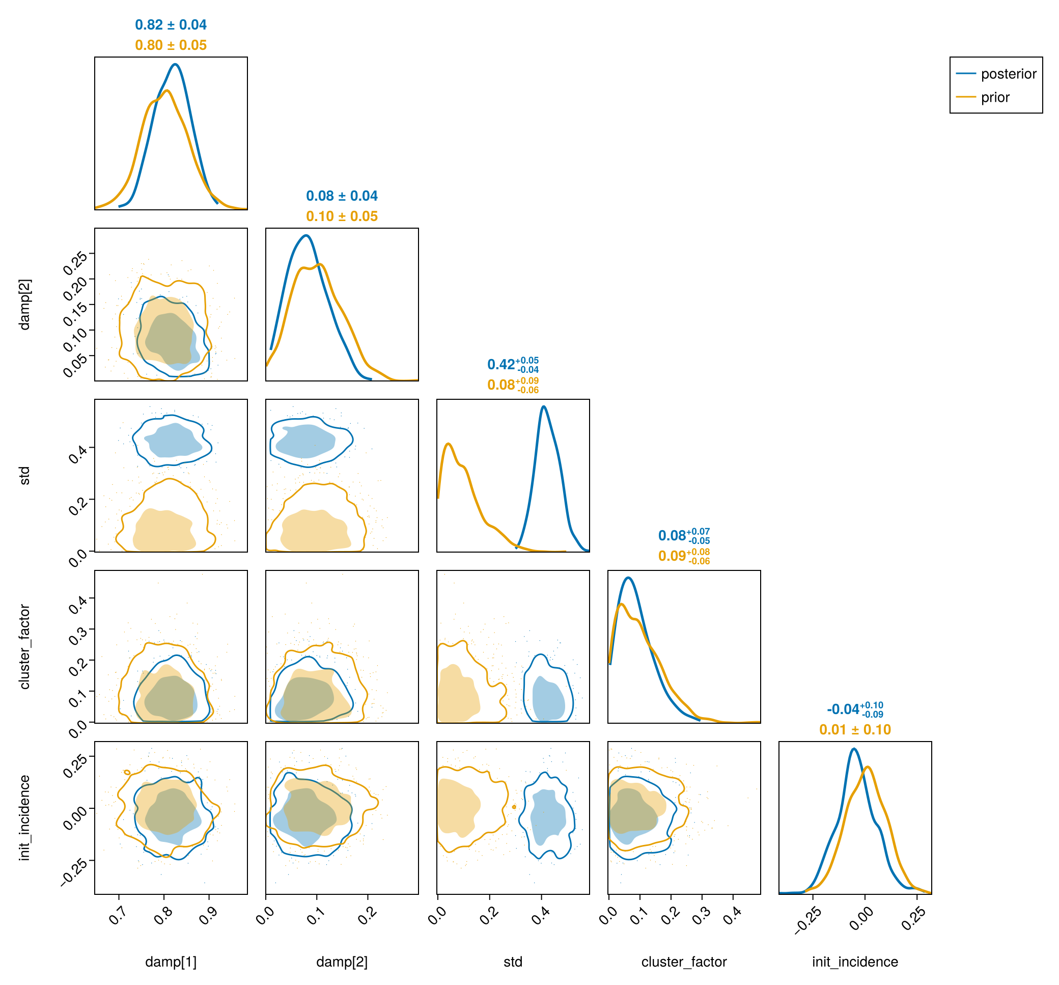
The innovation scale std) is sharply updated away from its prior, so the data are informative about how much damp), the cluster factor and the initial infections stay closer to their priors on this short window.
Posterior trajectories
The reproduction number generated_observables re-runs the fitted model over the chain to recover the latent predict on the same model with the observations set to missing.
A couple of small helpers reduce the per-draw trajectories to credible bands and draw a median line with 50% and 95% ribbons.
Stack the per-draw
gens = vec(generated_observables(posterior, y_obs, chain).generated)
Rt = credible_bands(reduce(hcat, (exp.(g.Z_t) for g in gens)))

pred = predict(as_turing_model(model, fill(missing, n), n), chain)
yt = predictive_bands(pred, n)

fig = Figure(; size = (760, 620))
ax1 = Axis(fig[1, 1]; ylabel = "Reproduction number Rₜ")
ci_ribbon!(ax1, 1:size(Rt, 1), Rt; color = :purple, label = "posterior median")
hlines!(ax1, [1.0]; color = :grey, linestyle = :dash)
axislegend(ax1; position = :rt)
ax2 = Axis(fig[2, 1]; xlabel = "Day", ylabel = "Reported cases")
ci_ribbon!(ax2, 1:size(yt, 1), yt; color = :teal,
    label = "posterior predictive")
scatter!(ax2, 1:n, y_obs; color = :black, markersize = 7, label = "observed")
axislegend(ax2; position = :lt)
fig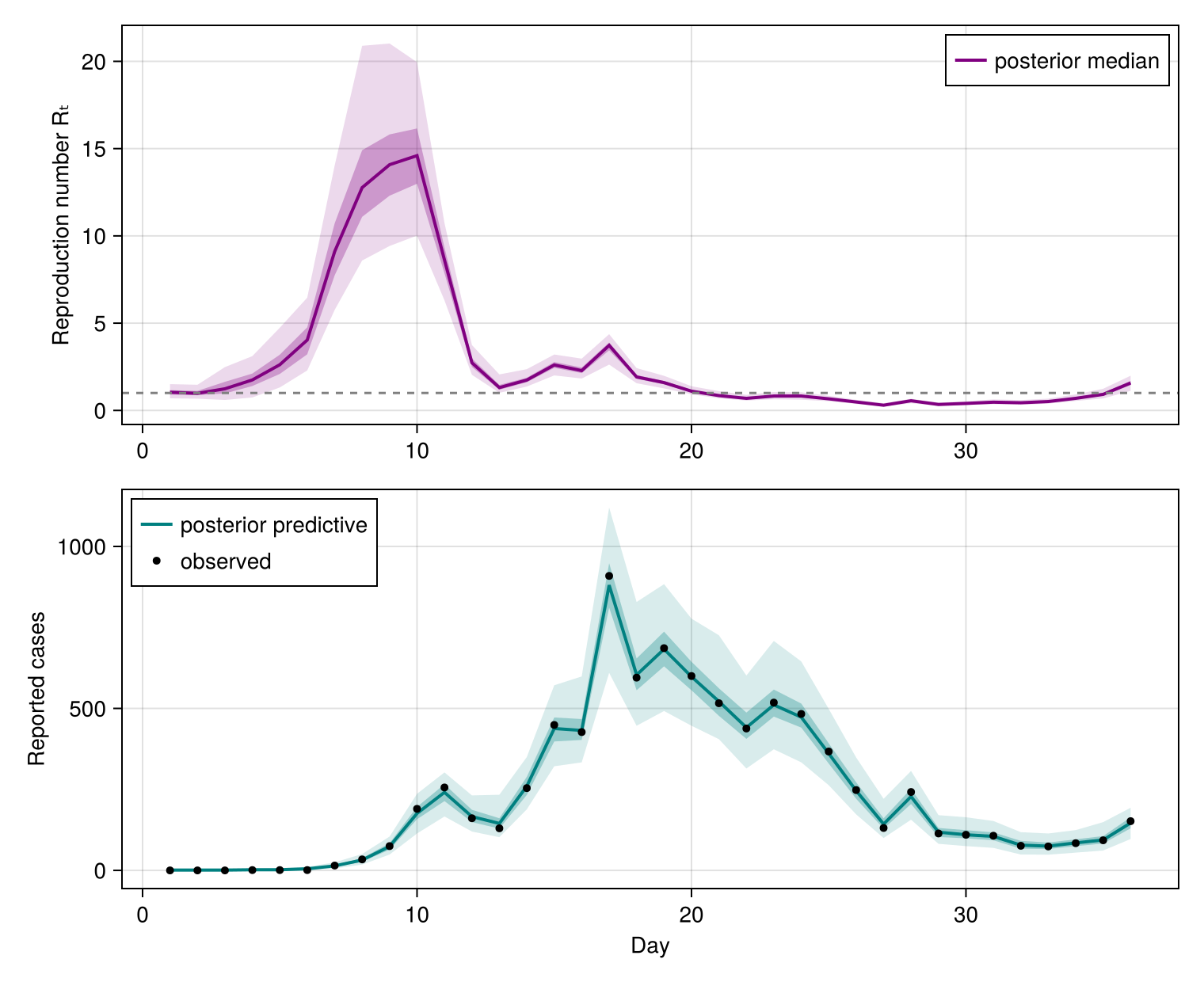
The posterior-predictive band tracks the observed South Korean series closely. The
Forecasting the next weeks
The same fitted model forecasts out of sample in one call. The latent AR process is non-centred, so forecast carries each posterior draw forward and then draws the future reported cases. It holds the fitted parameters and the in-sample
h = 14
fc = forecast(model, y_obs, chain, h)
round.(quantile(Float64.(vec(fc[@varname(y_t[n + h])])), [0.05, 0.5, 0.95]),
    digits = 1)
3-element Vector{Float64}:
6.0
302.5
50548.4The returned chain carries the predicted
# Multi-level CI band quantiles: 90%, 60%, 30% + median
FC_CI_QS = [0.05, 0.2, 0.35, 0.5, 0.65, 0.8, 0.95]

# Draw three nested CI ribbons with the median line
function multi_ci_ribbon!(ax, ts, bands; color, label)
    # 90% CI (cols 1, 7)
    band!(ax, ts, bands[:, 1], bands[:, 7]; color = (color, 0.1))
    # 60% CI (cols 2, 6)
    band!(ax, ts, bands[:, 2], bands[:, 6]; color = (color, 0.25))
    # 30% CI (cols 3, 5)
    band!(ax, ts, bands[:, 3], bands[:, 5]; color = (color, 0.5))
    # median (col 4)
    lines!(ax, ts, bands[:, 4]; color = color, linewidth = 2, label = label)
end

# Multi-level credible bands for the forecast
fc_bands = credible_bands(reduce(vcat,
    (permutedims(vec(fc[@varname(y_t[i])])) for i in (n + 1):(n + h)));
    qs = FC_CI_QS)

# Sample 100 random forecast trajectories
n_draws = length(vec(fc[@varname(y_t[n + 1])]))
ntraj = min(100, n_draws)
sample_idx = rand(1:n_draws, ntraj)
trajectories = reduce(hcat,
    [[vec(fc[@varname(y_t[i])])[idx] for i in (n + 1):(n + h)] for idx in sample_idx])

fig_fc = Figure(; size = (760, 360))
axf = Axis(fig_fc[1, 1]; xlabel = "Day", ylabel = "Reported cases",
    yscale = log10)
scatter!(axf, 1:n, y_obs; color = :black, markersize = 7, label = "observed")
# Faint individual forecast trajectories
for idx in 1:ntraj
    lines!(axf, (n + 1):(n + h), max.(trajectories[:, idx], 1);
        color = (:teal, 0.08), linewidth = 0.5)
end
# Multi-level CI bands (offset to keep log10 scale safe at zero)
multi_ci_ribbon!(axf, (n + 1):(n + h), max.(fc_bands, 1); color = :teal,
    label = "forecast")
vlines!(axf, [n + 0.5]; color = :grey, linestyle = :dash)
axislegend(axf; position = :lt)
fig_fc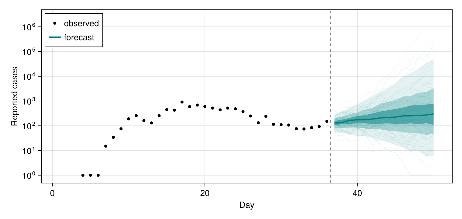
Swap a component
The parts share one interface, so an alternative observation assumption is a one-line change. Swapping the negative-binomial reporting for a PoissonError leaves the renewal infection process and its latent
using ComposableTuringIDModels: swap
poisson_model = swap(
    err -> err isa NegativeBinomialError ? PoissonError() : err, model)
IDModel
├─ infection: Renewal
│ └─ rt: AR
│ └─ ϵ_t: HierarchicalNormal
└─ observation: PoissonErrorswap walks the observation chain, replaces every component matching the predicate and rebuilds each wrapper around its replacement. See Inspecting and updating an observation chain for the general form, which also targets a single stream of a Split.
References
A. Cori, N. M. Ferguson, C. Fraser and S. Cauchemez. A new framework and software to estimate time-varying reproduction numbers during epidemics. American Journal of Epidemiology 178, 1505–1512 (2013).
S. Mishra, T. Berah, T. A. Mellan, H. J. Unwin, M. A. Vollmer, K. V. Parag, A. Gandy, S. Flaxman and S. Bhatt. On the derivation of the renewal equation from an age-dependent branching process: an epidemic modelling perspective, arXiv preprint arXiv:2006.16487 (2020).
K. Charniga, S. W. Park, A. R. Akhmetzhanov, A. Cori, J. Dushoff, S. Funk and others. Best practices for estimating and reporting epidemiological delay distributions of infectious diseases. PLoS Computational Biology 20, e1012520 (2024).