Time-varying damping in an AR process

Every parameter slot of a component takes a raw prior. Which kind of prior you put in the slot decides whether the parameter is constant or time-varying, through one mechanism any component can use.

• A bare Distribution gives a constant parameter, one scalar draw shared across the series with no length-n allocation.

• A process, a latent model such as a RandomWalk, gives a time-varying parameter, a whole path with one value per step.

The component reads the parameter the same way at every step with ComposableTuringIDModels.at(ρ, t), so a single recursion serves both cases. The damping coefficient of an autoregressive process is the worked example here, but the same widening applies to any scalar parameter.

Constant versus time-varying damping

AR with a Distribution damping prior is an ordinary constant-coefficient autoregression, with one number for the whole series.

using ComposableTuringIDModels, Distributions, Turing, Random, Statistics
using Mooncake
using ADTypes: AutoMooncake
Random.seed!(80)

constant = AR(; damp = Normal(0.4, 0.1))

AR
└─ ϵ_t: HierarchicalNormal

Swapping the Distribution for a process turns the same slot into a time-varying coefficient path .

where the unconstrained path is drawn from the process, a RandomWalk here, and tanh maps it into the stationary band  . This is a one-line change to the damp argument, leaving the AR recursion untouched.

tv = AR(; damp = RandomWalk())

AR
├─ damp: RandomWalk
│  └─ ϵ_t: HierarchicalNormal
└─ ϵ_t: HierarchicalNormal

transform is a field of AR, so the map is replaceable. It defaults to tanh for a process damp, which maps an unbounded draw into the stationary band  , and to identity for a Distribution, whose bounds are the user's to choose. The coefficient is transformed where it is drawn, so the recursion reads the mapped path.

Built with as_turing_model(m, n) it returns the numeric length-n path, as every other latent model does, and tracks the coefficient path as a generated quantity ρ.

as_turing_model(tv, 8)()

8-element Vector{Float64}:
  1.5842840380576646
 -0.23229794195656903
  0.05815398275952468
 -0.008276060914859553
 -0.006256093674879114
 -0.007622855895090526
 -0.008578701777191661
  0.005125758146265362

It returns a plain path, so it drops straight into any latent slot. Here that is the process of a Renewal inside a composed IDModel.

gen_int = [0.2, 0.3, 0.5]
nested = IDModel(
    Renewal(; generation_time = gen_int, rt = AR(; damp = RandomWalk()),
        initialisation = Normal()),
    PoissonError())
as_turing_model(nested, missing, 12)().generated_y_t

12-element Vector{Union{Missing, Int64}}:
 0
 4
 0
 0
 3
 5
 3
 6
 8
 3
 6
 8

We simulate one series whose true damping ramps from strong positive persistence through zero to mild anti-persistence, then recover it. A single series informs each through one transition, so recovery leans on the smoothness of the RandomWalk damping prior. A panel of series sharing one draw would sharpen it further.

n = 50
tgrid = range(0, 1; length = n - 1)
ρ_true = 0.85 .- 1.15 .* tgrid          # 0.85 → −0.30, crossing zero
z = zeros(n)
z[1] = randn()
for t in 2:n
    z[t] = ρ_true[t - 1] * z[t - 1] + 0.3 * randn()
end
(n = n, ρ_start = round(ρ_true[1], digits = 2),
    ρ_end = round(ρ_true[end], digits = 2))

(n = 50, ρ_start = 0.85, ρ_end = -0.3)

DirectInfections with transformation = identity and a fixed zero initialisation passes the AR path through as the expected series. A NormalError with a fixed standard deviation observes it. Fitting under NUTS recovers ρ from the chain. We draw two chains in parallel with MCMCThreads() and differentiate with Mooncake.

model = IDModel(
    DirectInfections(;
        Z = AR(; damp = RandomWalk()), transformation = identity,
        initialisation = FixedIntercept(0.0)),
    NormalError(; std = FixedIntercept(0.01)))
posterior = as_turing_model(model, z, n)
# Seed here, not only at the top: the simulation above consumes the stream, so
# an unrelated edit would otherwise move this fit's numbers.
Random.seed!(180)
fit = sample(
    posterior, NUTS(0.85; adtype = AutoMooncake(; config = nothing)),
    MCMCThreads(), 300, 2; progress = false)
ρ_draws = reduce(hcat, vec(fit[:ρ]))     # (n-1) × draws
ρ_mean = vec(mean(ρ_draws; dims = 2))
(correlation_with_truth = round(cor(ρ_mean, ρ_true), digits = 2),)

(correlation_with_truth = 0.75,)

The posterior median damping path tracks the true ramp, including the sign change.

using CairoMakie
qs = [quantile(ρ_draws[t, :], [0.1, 0.5, 0.9]) for t in 1:(n - 1)]
lo = getindex.(qs, 1)
md = getindex.(qs, 2)
hi = getindex.(qs, 3)

fig = Figure(; size = (760, 420))
ax = Axis(fig[1, 1]; xlabel = "Time step", ylabel = "Damping ρₜ")
band!(ax, 1:(n - 1), lo, hi; color = (:seagreen, 0.25))
lines!(ax, 1:(n - 1), md; color = :seagreen, linewidth = 2,
    label = "posterior median")
lines!(ax, 1:(n - 1), ρ_true; color = :black, linestyle = :dash, linewidth = 2,
    label = "true ρₜ")
hlines!(ax, [0.0]; color = :grey, linestyle = :dot)
axislegend(ax; position = :lb)
fig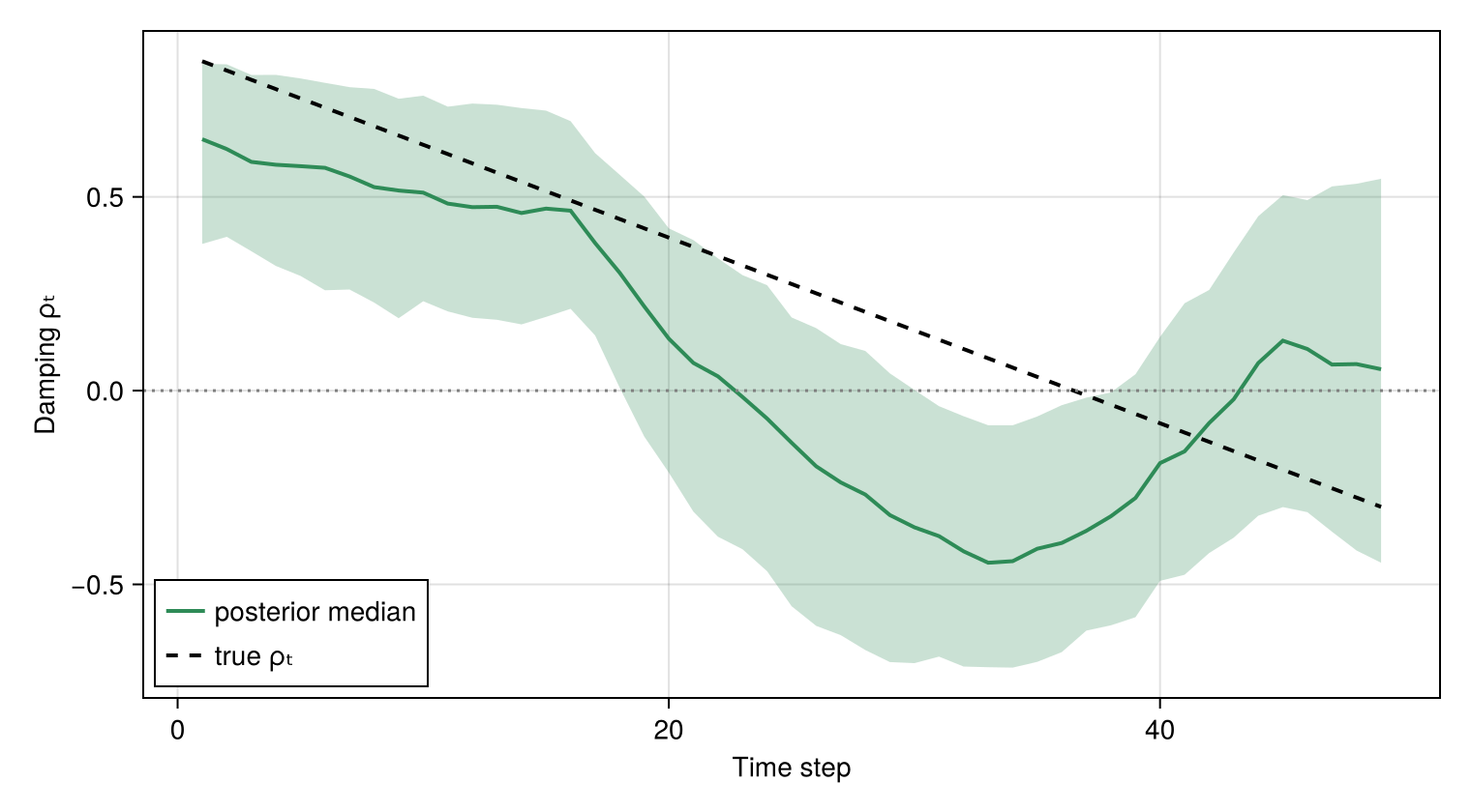

The band covers the true trajectory across the series, so the time-varying damping is recovered from data. Only the order-1 case is built so far. Time-varying coefficients for a higher-order AR(p) are not built yet.

Nothing about this is specific to AR. arma takes the same damp slot, and DiffLatentModel differences whatever it wraps, so a time-varying-damping ARIMA is the two of them composed.

arima_tv = arima(; damp = RandomWalk(), diff_init = [Normal(0.3, 0.3)])

DiffLatentModel
└─ model: AR
   ├─ damp: RandomWalk
   │  └─ ϵ_t: HierarchicalNormal
   └─ ϵ_t: MA
      └─ ϵ_t: HierarchicalNormal